6 Bayesian tools for machine learning
This chapter covers
- Unsupervised machine learning models
- Bayes’ theorem, conditional probability, entropy, cross-entropy, and conditional entropy
- Maximum likelihood estimation (MLE) and maximum a posteriori (MAP) estimation of model parameters
- Evidence maximization
- KLD
- Gaussian mixture models (GMM) and MLE estimation of GMM parameters
The Bayesian approach to statistics tries to model the world by modeling the uncertainties and prevailing beliefs and knowledge about the system. This is in contrast to the frequentist paradigm, where probability is strictly measured by observing a phenomenon repeatedly and measuring the fraction of time an event occurs. Machine learning, in particular unsupervised machine learning, is a lot closer to the Bayesian paradigm of statistics—the subject of this chapter.
In chapter 1, we primarily discussed supervised machine learning, where the training data is labeled: each input value is accompanied by a manually created desired output value. Labeling training inputs is a manual, labor-intensive process and often the worst pain point in building a machine learning–based system. This has led to considerable recent interest in unsupervised machine learning, where we build a model from unlabeled training data. How is this done?
The general approach is best visualized geometrically. Each input data instance is a point in a high-dimensional space. These points form an overall pattern in the space of all possible inputs. If the inputs all have a common property, the points are not distributed randomly over the input space. Rather, they occupy a region in the input space with a definite shape. If the inputs have multiple classes, each class occupies a separate cluster in the space. Sometimes we apply a transformation to the input first—the transform is chosen or learned so that the transformed points exhibit a pattern more clearly than raw input points. We then identify a probability distribution whose sample point cloud matches the shape of the (potentially transformed) training data point cloud. We can generate faux input by sampling from this distribution. We can also classify an arbitrary input by observing which cluster it falls into.
NOTE The complete PyTorch code for this chapter is available at http://mng.bz /WdZa in the form of fully functional and executable Jupyter notebooks.
6.1 Conditional probability and Bayes’ theorem
As usual, the discussion is accompanied by examples. In this context, we first offer a refresher on the concepts of joint and marginal probability from section 5.4 (you may want to revisit the topic of joint probability in sections 5.4, 5.4.1, and 5.4.2).
Consider two random variables: the height and weight of adult Statsville residents. Weight (denoted W) can take three quantized values: E1, E2, E3. Height (H) can also take three quantized values: F1, F2, F3. Table 6.1 shows their joint probability.
6.1.1 Joint and marginal probability revisited
One glance at table 6.1 tells us that the probabilities are concentrated along the main diagonal, which indicates dependent events. This can be validated by inspecting one joint probability—say, p(E1, F1)—and the corresponding marginal probabilities p(F1) and p(E1). We can see that p(E1, F1) = 0.2 ≠ p(F1) × p(E1) = 0.26 × 0.26, establishing that the random variables weight W and height H are not independent. For contrast, look at table 5.6. In that case, for any valid i, j pair, p(Ei, Gj) = p(Gi) × p(Ej): the two events (weight and distance of a resident’s home from the city center) are independent. Note the following:
Table 6.1 Example population sizes and joint probability distribution for variables W = {E1, E2, E3} and H = {F1, F2, F3} weights and heights of adult Statsville residents), showing marginal probabilities
|
Less than 60 kg (E1) |
Between 60 and 90 kg (E2) |
More than 90 kg (E3) |
Marginals for Fs |
|
|---|---|---|---|---|
|
Less than 160 cm (F1) |
pop. = 20,000 p(E1, F1) = 0.2 |
pop. = 4,000 p(E2, F1) = 0.04 |
pop. = 2,000 p(E3, F1) = 0.02 |
pop. = 26,000; p(F1) = 0.2 + 0.04 + 0.02 = 0.26 |
|
Between 160 cm and 183 cm (F2) |
pop. = 4,000 p(E1, F2) = 0.04 |
pop. = 40,000 p(E2, F2) = 0.4 |
pop. = 4,000 p(E3, F2) = 0.04 |
pop. = 48,000; p(F2) = 0.04 + 0.4 + 0.04 = 0.48 |
|
More than 183 cm (F3) |
pop. = 2,000 p(E1, F3) = 0.02 |
pop. = 4,000 p(E2, F3) = 0.04 |
pop. = 20,000 p(E3, F3) = 0.2 |
pop. = 26,000; p(F3) = 0.02 + 0.04 + 0.2 = 0.26 |
|
Marginals for Es |
p(E1) = 0.2 + 0.04 + 0.02 = 0.26 |
p(E2) = 0.04 + 0.4 + 0.04 = 0.48 |
p(E3) = 0.02 + 0.04 + 0.2 = 0.26 |
Total pop. = 100,000; Total prob = 1 |
-
Joint probability—This is the probability of a specific combination of values occurring together. Each cell in table 6.1 depicts one joint probability: for example, the probability that a resident’s weight is between 60 and 90 kg and that their height is greater than 183 cm is p(E2, F3) = 0.04.
-
Sum rule—The joint probabilities of all possible variable combinations sum to 1 (bottom right cell in table 6.1):
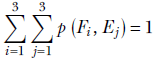
The sum of probabilities is the probability of one or another of the corresponding events occurring. Here we are adding all possible event combinations—one or another of these combinations will certainly occur. Hence the sum is 1, which matches our intuition.
-
Marginal probability for a variable—This is obtained by “summing away” the other variables (right-most column and bottom-most row in table 6.1):
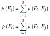
We have added all possible combinations of other variables, so the sum represents the probability of this one variable.
-
Marginal probabilities—These sum to 1:
The sum of the marginal probabilities is the sum of all possible joint probabilities.
-
Dependent vs. independent variables—If and only if the variables are independent, the product of the marginal probabilities is the same as the joint probability:
p(Fi , Ej) ≠ p(Fi) × p(Ej) ⟺ for dependent variables in table 5.6
p(Gi , Ej) = p(Gi) × p(Ej) ⟺ for independent variables in table 6.1
You should verify that this condition is not satisfied in table 6.1 for the weight and height variables. It is satisfied in table 5.6 for the weight and distance-of-home-from-city-center variables.
6.1.2 Conditional probability
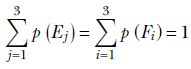
Suppose we know that the height of a subject is between 160 and 183 cm (H = F2). What is the probability of the subject’s weight being more than 90 kg (W = E3)? In statistical parlance, this probability is denoted p(W = E3|H = F2). It is read “probability of W = E3 given H = F2,” aka “probability of W = E3 subject to the condition H = F2.”
This is an example of conditional probability. Note that if we are given that the height is between 160 and 183 cm (H = F2), our universe is restricted to the second row of table 6.1. In particular, our population size is not 100,000 (that is, the entire population of Statsville). Rather, it is 48,000: the size of the population satisfying the given condition H = F2. Using the frequentist definition,
Table 6.2 shows table 6.1 with conditional probabilities added.
Table 6.2 Example population sizes and joint, marginal, and conditional probabilities for variables W = {E1, E2, E3} and H = {F1, F2, F3} weights and heights of adult Statsville residents). (This is table 6.1 with conditional probabilities added.)
|
Less than 60 kg (E1) |
Between 60 and 90 kg (E2) |
More than 90 kg (E3) |
Marginals for Fs |
|
|---|---|---|---|---|
|
Less than 160 cm (F1) |
pop. = 20,000 p(E1, F1) = 0.2 p(E1| F1) = p(E1, F1) / p(F1) = 0.77 p(F1| E1) = p(E1, F1) / p(E1) = 0.77 |
pop. = 4,000 p(E2, F1) = 0.04 p(E2| F1) = p(E2, F1) / p(F1) = 0.154 p(F1| E2) = p(E2, F1) / p(E2) = 0.083 |
pop. = 2,000 p(E3, F1) = 0.02 p(E3| F1) = p(E3, F1) / p(F1) = 0.077 p(F1| E3) = p(E3, F1) / p(E3) = 0.077 |
pop. = 26,000; p(F1) = 0.2 + 0.04 + 0.02 = 0.26 |
|
Between 160 cm and 183 cm (F2) |
pop. = 4,000 p(E1, F2) = 0.04 p(E1| F2) = p(E1, F2) / p(F2) = 0.083 p(F2)| E1) = p(E1, F2) / p(E1) = 0.154 |
pop. = 40,000 p(E2, F2) = 0.4 p(E2| F2) = p(E2, F2) / p(F2) = 0.83 p(F2)| E2) = p(E2, F2) / p(E2) = 0.83 |
pop. = 4,000 p(E3, F2) = 0.04 p(E3| F2) = p(E3, F2) / p(F2) = 0.083 p(F2)| E3) = p(E3, F2) / p(E3) = 0.154 |
pop. = 48,000; p(F2) = 0.04 + 0.4 + 0.04 = 0.48 |
|
More than 183 cm (F3) |
pop. = 2,000 p(E1, F3) = 0.02 p(E1|F3) = p(E1, F3) / p(F3) = 0.077 p(F3|E1) = p(E1, F33) / p(E1) = 0.077 |
pop. = 4,000 p(E2, F3) = 0.04 p(E2|F3) = p(E2, F3) / p(F3) = 0.154 p(F3|E2) = p(E2, F33) / p(E2) = 0.083 |
pop. = 20,000 p(E3, F3) = 0.2 p(E3|F3) = p(E3, F3) / p(F3) = 0.77 p(F3|E3) = p(E3, F33) / p(E3) = 0.77 |
pop. = 26,000; p(F3) = 0.02 + 0.04 + 0.2 = 0.26 |
|
Marginals for Es |
p(E1) = 0.2 + 0.04 + 0.02 = 0.26 |
p(E2) = 0.04 + 0.4 + 0.04 = 0.48 |
p(E3) = 0.02 + 0.04 + 0.2 = 0.26 |
Total pop.= 100,000; Total prob = 1 |
6.1.3 Bayes’ theorem
As demonstrated in table 6.2, in general,
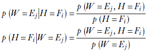
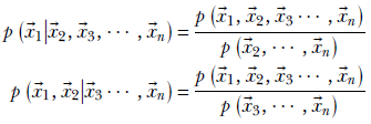
This is the essence of Bayes’ theorem. We can generalize and say the following: given two random variables X and Y, the conditional probability of X taking the value x given the condition that Y has value ![]() is given by the ratio of the joint probability of the two and the marginal probability of the condition
is given by the ratio of the joint probability of the two and the marginal probability of the condition
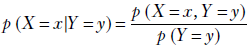
Equation 6.1
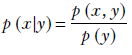
Sometimes we drop the names of the random variable and just use the values. Using such notation, Bayes’ theorem can be stated as
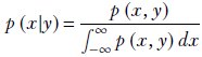
Note that the denominator is the marginal probability, which can be obtained by summing over the joint probabilities. For instance, for continuous variables, Bayes’ theorem can be written as
Bayes’ theorem can be generalized further to more than two variables and multiple dimensions:

Equation 6.2

Equation 6.3
It is common practice to drop the name of the random variable uppercase), retain only the value (lowercase), and state these equations informally as
What happens if the random variables are independent? Well, let’s check out equation 6.1. If X and Y are independent,
![]()
and hence
![]()
This makes intuitive sense: if X and Y are independent, knowing Y does not make any difference to p(X = x), so the probability of X given Y is the same as the probability of X.
6.2 Entropy
Suppose a daily meteorological bulletin informs the folks in the United States whether it rained in the Sahara desert yesterday. Is there much overall information in that bulletin? Not really—it almost always reports the obvious. The probability of “no rain” is overwhelmingly high it is almost certain that there will be no rain), and the uncertainty associated with the outcome is very low. Even without the bulletin, if we guess the outcome “no rain,” we will be right almost every time. Similarly, a daily news bulletin telling us whether it rained yesterday in Cherapunji, India—a place where it pretty much rains all the time—has little informational content because we can guess the results with high certainty even without the bulletin. Stated another way, the uncertainty associated with the probability distributions of “rain vs. no rain in the Sahara” and or “rain vs. no rain in Cherapunji” is low. This is a direct consequence of the fact that the probability of one of the events is close to 1 and the probabilities of the other events are near 0: the probability density function (PDF) has a very tall peak at one location and very low heights elsewhere.
On the other hand, a daily bulletin reporting whether it rained in San Francisco is of considerable interest because the probability of “rain” and “no rain” are comparable. Without the bulletin, we cannot guess the result with much certainty.
The concept of entropy attempts to quantify the uncertainty associated with a chancy event. If the probability for any one event is overwhelmingly high (meaning the probabilities of other events are very low since the sum is 1), the uncertainty is low—we pretty much know that the high-probability event will occur. On the other hand, if there are multiple events with comparable high probabilities, uncertainty is high—we cannot predict which event will occur. Entropy captures this notion of uncertainty in a system. Let’s look at another example.
Suppose we have tiny images, four pixels wide by four pixels high, and each pixel is one of four possible colors: G(reen), R(ed), B(lue), or Y(ellow). Two such images are shown in figure 6.1. We want to encode such images. The simplest thing to do is to use a two-bit representation for each color:
G(reen) = 00
R(ed) = 01
B(lue) = 10
Y(ellow) = 11
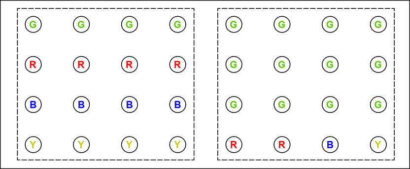
Figure 6.1 Two 4 × 4 images with different pixel color distributions. In the left image, the four colors R, G, B, and Y are equally probable. In the right image, one color (green) is much likelier than the others. The left image has higher entropy (uncertainty): we cannot predict any color with much certainty. In the right image, we can predict green with relative certainty.
The entire 16-pixel image on the left can be represented by the string 00 00 00 00 01 01 01 01 10 10 10 10 11 11 11 11. Here, we have iterated over the pixels in raster scan order, left to right and top to bottom. The total number of bits needed to store the 16-pixel image is 16 × 2 = 32 bits. The right image can be represented as 00 00 00 00 00 00 00 00 00 00 00 00 01 01 10 11. The total number of bits needed is 16 × 2 = 32 bits. Both images need the same amount of storage. But is this optimal?
Consider the right-hand image. The color G appears much more frequently than the others. We can use this fact to reduce the total number of bits required to store the image. It is not mandatory to use the same number of bits to represent each color. How about using shorter representations for the more frequently occurring (higher-probability) colors and longer representations for the infrequent (lower-probability) colors? This is the core principle behind the technique of variable bit-rate coding. For instance, we can use the following representation:
G(reen) = 0
R(ed) = 10
B(lue) = 110
Y(ellow) = 111
The right-hand image can thus be represented as 0 0 0 0 0 0 0 0 0 0 0 0 10 10 110 111.
NOTE This is an example of what is known as prefix coding: no two colors share the same prefix. It enables us to identify the color as soon as we see its code. For instance, if we see a 0 bit at the beginning, we immediately know the color is green since no other color code starts with 0. If we see 10, we immediately know the color is red since no other color code starts with 10, and so on.
With this new color code, we need 12 × 1 = 12 bits to store the 12 green pixels, 2 × 2 = 4 bits to store the 2 red pixels, 1 × 3 = 3 bits to store the single blue pixel, and 1 × 3 = 3 bits to store the single yellow pixel—a total of 22 pixels. Equivalently, we need 22/16 = 1.375 bits per pixel. This is less than the 32 pixels at 2 bits per pixel we needed with the simple fixed bit-rate coding.
NOTE You have just learned about Huffman encoding, an important technique in image compression.
Does the new representation result in smaller storage for the left-hand image? There, we need 4 × 1 = 4 bits to store the four green pixels, 4 × 2 = 8 pixels to store the four red pixels, 4 × 3 = 12 bits to store the four blue pixels, and 4 × 3 = 12 bits to store the single yellow pixel: a total of 36 pixels at 36/16 = 2.25 bits per pixel. Here, variable bit-rate coding does worse than fixed bit-rate coding.
So, the probability distribution of the various pixel colors in the image affects how much compression can be achieved. If the distribution of pixel colors is such that a few colors are much more probable than others, we can assign shorter codes to them to reduce storage for the whole image. Viewed another way, if low uncertainty is associated with the system—certain colors are more or less certain to occur—we can achieve high compression. We assign shorter codes to nearly certain colors, resulting in compression. On the other hand, if high uncertainty is associated with the system—all colors are more or less equally probable, and no color occurs with high certainty—variable bit-rate coding will not be very effective. How do we quantify this notion? In other words, can we examine the pixel color distribution in an image and estimate whether variable bit-rate coding will be effective? The answer again is entropy. Formally,
Entropy measures the overall uncertainty associated with a probability distribution.
Entropy is a measure that is high if everything is more or less equally probable and low if a few items have a much higher probability than the others. It measures the uncertainty in the system. If everything is equally probable, we cannot predict any one item with any extra certainty. Such a system has high entropy. On the other hand, if some items are much more probable than others, we can predict them with relative certainty. Such a system has low entropy.
In the discrete univariate case, for a random variable X that can take any one of the discrete values x1, x2, x3, ⋯, xn with probabilities p(x1), p(x2), p(x3), ⋯, p(xn), entropy is defined as
Equation 6.4
The logarithm is taken with respect to the natural base e.
Let’s apply equation 6.4 to the images in figure 6.1 to see if the results agree with our intuition. The computations are shown in table 6.3. The notion of entropy applies to continuous and multidimensional random variables equally well.
Table 6.3 Entropy computation for the pair of images in figure 6.1. The right-hand image has lower entropy and can be compressed more.
|
Left image |
Right image |
|---|---|
|
x1 = G, p(x1) = 4/16 = 0.25 |
x1 = G, p(x1) = 12/16 = 0.75 |
|
x2 = R , p(x2) = 4/16 = 0.25 |
x2 = R , p(x2) = 2/16 = 0.125 |
|
x3 = B, p(x3) = 4/16 = 0.25 |
x3 = B, p(x3) = 1/16 = 0.0625 |
|
x4 = Y, p(x4) = 4/16 = 0.25 |
x4 = Y, p(x4) = 1/16 = 0.0625 |
|
ℍ = −(0.25 log(0.25)+0.25 log(0.25) + |
ℍ = −(0.75 log(0.75)+0.125 log(0.125) + |
For a univariate continuous random variable X that takes values x ∈ {−∞,∞} with probabilities p(x),
Equation 6.5
For a continuous multidimensional random variable X that takes values ![]() in the domain D, (
in the domain D, (![]() ∈ D) with probabilities p(
∈ D) with probabilities p(![]() ),
),
Equation 6.6
6.2.1 Geometrical intuition for entropy
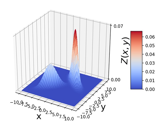
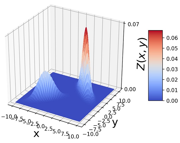
Geometrically speaking, entropy is a function of how lopsided the PDF is (see figure 6.2). If all inputs are more or less equally probable, the density function is more or less flat and uniform in height everywhere (see figure 6.2a). The corresponding sample point cloud has a diffused mass: there are no regions with a high concentration of points. Such a system has high uncertainty or high entropy (see figure 6.2b).
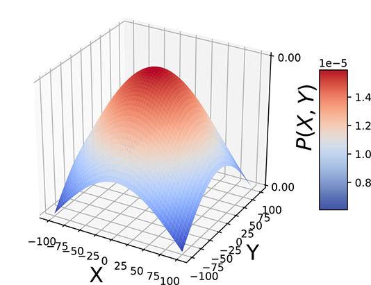
(a) Flatter, wider PDFs correspond to higher entropy. Entropy = 12.04.
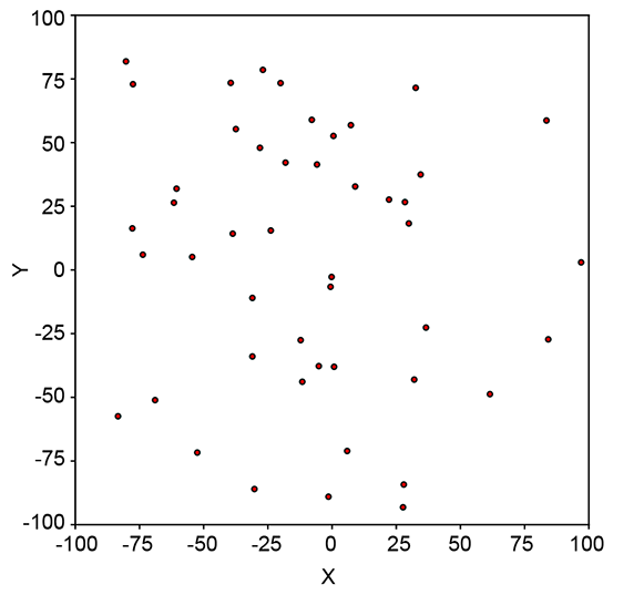
(b) Diffused sample point clouds correspond to higher entropy.
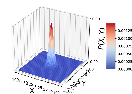
(c) Taller, narrower peaks in probability density functions correspond to lower entropy. Entropy = 7.44.
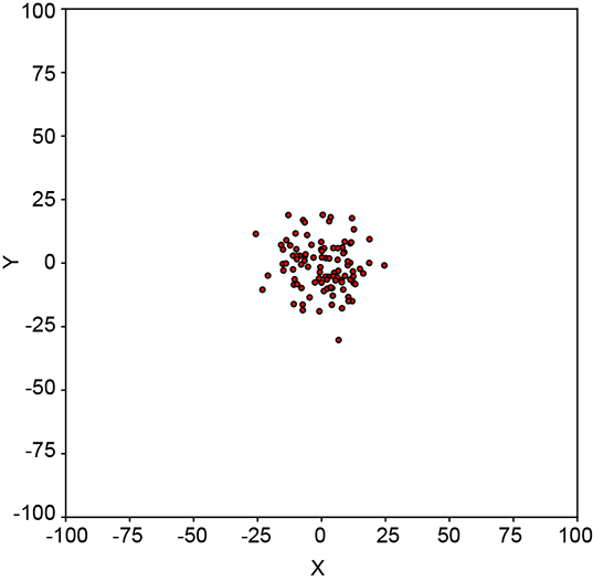
(d) Concentrated sample point clouds correspond to lower entropy.
Figure 6.2 Entropies of peaked and flat distributions
On the other hand, if a few of all the possible inputs have disproportionately high probabilities, the PDF has tall peaks in some regions and low heights elsewhere (see figure 6.2c). The corresponding sample point cloud has regions of high concentration matching the peaks in the density function and low concentration elsewhere (see figure 6.2d). Such a system has low uncertainty and low entropy.
NOTE Since the sum of all the probabilities is 1, if a few are high, the others have to be low. We cannot have all high or all low probabilities.
6.2.2 Entropy of Gaussians
The wider a Gaussian is, the less peaked it is, and the closer it is to being a uniform distribution. A univariate Gaussian’s variance, σ, determines its fatness (see figure 5.10b). Consequently, we expect a Gaussian’s entropy to be an increasing function of σ. Indeed, that is the case. In this section, we derive the entropy of a Gaussian in the univariate case and simply state the result for the multivariate case.
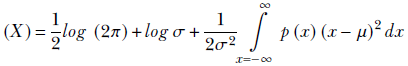
For a random variable x whose PDF is given by equation 5.22 (repeated here for convenience),
From that, we get
Using equation 6.6, the entropy is
Remembering the probability sum rule from equation 5.6, ∫x = −∞∞ p(x) dx = 1, we get
Now, by definition (see section 5.7.2),
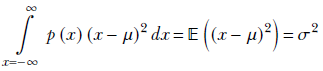
Hence,

Equation 6.7
Entropy for multivariate Gaussians is as follows:
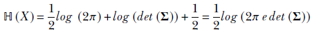
Equation 6.8
Listing 6.1 shows the Python PyTorch code to compute the entropy of a Gaussian.
NOTE Fully functional code to compute the entropy of a Gaussian distribution, executable via Jupyter Notebook, can be found at http://mng.bz/zx7B.
Listing 6.1 Computing the entropy of a Gaussian distribution
def entropy_gaussian_formula(sigma):
    return 0.5 * torch.log(2 * math.pi * math.e * sigma * sigma) ①

p = Normal(0, 10)                                                ②

H_formula = entropy_gaussian_formula(p.stddev)                   ③

H = p.entropy()                                                  ④

assert torch.isclose(H_formula, H)                               ⑤
① Equation 6.7
② Instantiates a Gaussian distribution
③ Computes the entropy using the direct formulaComputes the entropy using the direct formula
④ Computes the entropy using the PyTorch interface
⑤ Asserts that the entropies computed two different ways match
6.3 Cross-entropy
Consider a supervised classification problem where we have to analyze an image and identify which of the following objects is present: cat, dog, airplane, or automobile. We assume that one of these will always be present in our universe of images. Given an input image, our machine emits four probabilities: p(cat), p(dog), p(airplane), and p(automobile). During training, for each training data instance, we have a ground truth (GT): a known class to which that training data instance belongs. We have to estimate how different the network output is from the GT—this is the loss for that data instance. We adjust the machine parameters to minimize the loss and continue doing so until the loss stops decreasing.
How do we quantitatively estimate the loss—the difference between the known GT and the probabilities of various classes emitted by the network? One principled approach is to use the cross-entropy loss. Here is how it works.
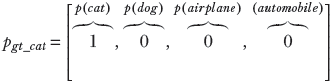
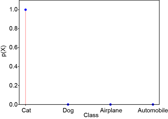
Consider a random variable X that can take four possible values: X = 1 signifying cat, X = 2 signifying dog, X = 3 signifying airplane, and X = 4 signifying automobile. The random variable has the PDF p(X = 1) ≡ p(cat), p(X = 2) ≡ p(dog), p(X = 3) ≡ p(airplane), p(X = 4) ≡ p(automobile). The PDF for a GT, which selects one from the set of four possible classes, is a one-hot vector (one of the elements is 1, and the others are 0). Such random variables and corresponding PDFs can be associated with every GT and machine output. Here are some examples, which are also shown graphically in figure 6.3. A PDF for GT cat (one-hot vector) is shown figure 6.3a:
How do we quantitatively estimate the loss—the difference between the known GT and the probabilities of various classes emitted by the network? One principled approach is to use the cross-entropy loss. Here is how it works.
A PDF for a good prediction is shown figure 6.3b:
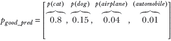
A PDF for a bad prediction is shown figure 6.3c:
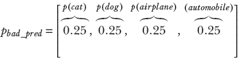
(a) Ground truth probability
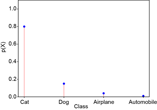
(b) Good prediction: probabilities similar to ground truth. Cross-entropy loss = 0.22.
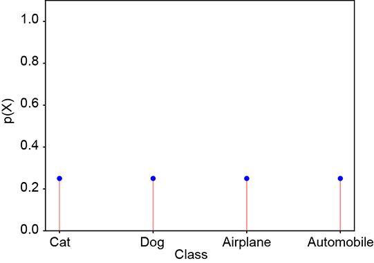
(c) Bad prediction: probabilities dissimilar to ground truth. Cross-entropy loss = 1.38.
Figure 6.3 Cross-entropy loss
Let Xgt denote such a random variable for a specific GT and pgt denote the corresponding PDF. Similarly, let Xpred and ppred denote the random variable and PDF for the machine prediction. Consider the following expression:
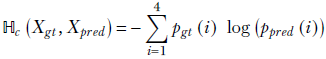
Equation 6.9
This is the expression for cross-entropy. It is a quantitative measure for how dissimilar the two PDFs pgt and ppred are: that is, how much error will be caused by approximating the PDF pgt with ppred. Equivalently, cross-entropy measures how well the machine is doing that output the prediction ppred when the correct PDF is pgt.
To gain insight into how ℍc(Xgt, Xpred) measures dissimilarity between PDFs, examine the expression carefully. Remember that Σi4= 1 pgt (i) = Σi4= 1 ppred (i) = 1 (using the probability sum rule from equation 5.3):
Case 1: The i values where pgt(i) is high (close to 1).
Case 1a: If ppred(i) is also close to 1, then log (ppred(i)) will be close to zero (since log 1 = 0). Hence the term pgt(i)log (ppred(i)) will be close to zero since the product of anything with a near-zero number is near zero. These terms will contribute little to ℍc(Xgt, Xpred).
Case 1b: On the other hand, at the i values where pgt(i) is high, if ppred(i) is low (close to zero), then −log (ppred(i)) will be very high (since log 0 → − ∞).
Case 2: The i values where pgt(i) is low (close to 0). These will have low values and will contribute little to ℍc(Xgt, Xpred) since the product of anything with a near zero number is near zero.
Thus, overall, large contributions can happen only in case 1b, where pgt(i) is high and ppred(i) is low—that is, pgt and ppred are very dissimilar. What if pgt(i) is low and ppred(i) is high? They are also dissimilar, so those terms will not contribute much! True, but if such terms exist, there must be other terms where pgt(i) is high and ppred(i) is low. This is because the sums of all pgt(i) and ppred(i) must be both 1. Either way, if there is dissimilarity, the cross-entropy is high.
For instance, consider the case where Xgt = Xgt_cat and Xpred = Xgood_pred or Xpred = Xbad_pred. We know pgt_cat is a one-hot selector vector, meaning it has 1 as one element and 0s elsewhere. Only a single term survives, corresponding to i = 0, and
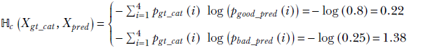
We see that cross-entropy is higher where similarity is lower (the prediction is bad).
Finally, we are ready to formally define the cross-entropy of two arbitrary random variables. Let X1, X2 be a pair of random variables that take values x from the same input domain D that is, x ∈ D), with probabilities p1(x), p2(x), respectively:
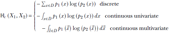
Equation 6.10
Note that cross-entropy in equation 6.10 reduces to entropy (equations 6.5, 6.6) if Y = X. Listing 6.2 shows the Python PyTorch code to compute the entropy of a Gaussian.
NOTE Fully functional code to compute cross-entropy, executable via Jupyter Notebook, can be found at http://mng.bz/0mjN.
Listing 6.2 Computing cross-entropy
def cross_entropy(X_gt, X_pred):
    H_c = 0
    for x_gt, x_pred in zip(X_gt, X_pred):
        H_c += -1 * (x_gt * torch.log (x_pred))     ①
    return H_c

X_gt = torch.Tensor([1., 0., 0., 0.])               ②

X_good_pred = torch.Tensor([0.8, 0.15, 0.04, 0.01]) ③

X_bad_pred = torch.Tensor([0.25, 0.25, 0.25, 0.25]) ④

H_c_good = cross_entropy(X_gt, X_good_pred)         ⑤

H_c_bad = cross_entropy(X_gt, X_bad_pred)           ⑥
① Direct computation
of cross-entropy from equation 6.9
② Probability density function for the ground truth (one-hot vector)
③ Probability density function for a good prediction
④ Probability density function for a bad prediction
⑤ Cross-entropy between Xgt and Xgood_pred a low value)
⑥ Cross-entropy between Xgt and Xbad_pred a high value)
6.4 KL divergence
In section 6.3, we saw that cross-entropy, ℍc(X1, X2), measures the dissimilarity between the distributions of two random variables X1 and X2 with probabilities p1(x) and p2(x). But cross-entropy has a curious property for a dissimilarity measure. If X1 = X2, the cross-entropy ℍc(X1, X2) reduces to the entropy ℍ(X1). This is somewhat counterintuitive: we expect the dissimilarity between two copies of the same thing to be zero.
We should look at cross-entropy as a dissimilarity with an offset. Let’s denote the pure dissimilarity measure as D(X1, X2). Then
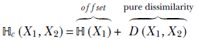
This means the pure dissimilarity measure
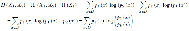
This pure dissimilarity measure, D(X1, X2), is called Kullback–Leibler divergence (KL divergence or KLD). As expected, it is 0 when the two random variables are identical.
Formally, KLD is as follows:
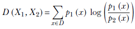
Equation 6.11
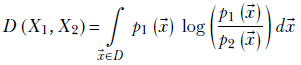
For continuous univariate randoms,
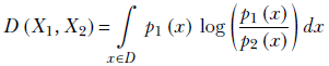
Equation 6.12
For continuous multivariate randoms,
Equation 6.13
Let’s examine some properties of KLD:
-
The KLD between identical random variables is zero. If X1 = X2, p1(x) = p2(x)∀x ∈ D. Then the log term vanishes at every x, and KLD is zero.
-
The KLD between non-identical probability distributions is always positive. We can see this by examining equation 6.11. At all values of x where p1(x) > p2(x), the log term is positive (since the logarithm of a number greater than 1 is positive). On the other hand, at all values of x where p1(x) < p2(x), the log term is negative (since the logarithm of a number less than 1 is negative). But the positive terms get higher weights because p1(x) are higher at these points. In this context, it is worth noting that given any pair of PDFs, one cannot be uniformly higher than the other at all points. This is because both of them must sum to 1. If one PDF is higher somewhere, it must be lower somewhere else to compensate.
-
Given a GT PDF pgt for a classification problem and a machine prediction ppred, minimizing the cross-entropy ℍ(gt, pred) is logically equivalent to minimizing the KLD D(gt, pred). This is because the entropy ℍ(gt) is a constant, independent of the machine parameters.
-
The KLD is not symmetric: D(X1, X2) ≠ D(X2, X1).
6.4.1 KLD between Gaussians
Since the Gaussian probability distribution is so important, in this subsection we look at the KLD between two Gaussian random variables X1 and X2 having PDFs p1(x) = 𝒩(x; μ1, σ1) and p2(x) = 𝒩(x; μ2, σ2). We derive the expression for the univariate case and simply state the expression for the multivariate case:
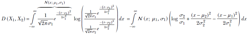
Opening the parentheses, we get

Expanding the square term, we get

Since
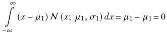
the final equation for the KLD between two univariate Gaussian random variables X1, X2 with PDFs 𝒩(x; μ1, σ1) and 𝒩(x; μ2, σ2) becomes
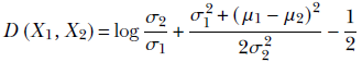
Equation 6.14
The KLD between two d-dimensional Gaussian random variables X1, X2 with PDFs 𝒩(![]() ; μ1, Σ1) and 𝒩(
; μ1, Σ1) and 𝒩(![]() ; μ2, Σ2) is
; μ2, Σ2) is

Equation 6.15
where the operator tr denotes the trace of a matrix (sum of diagonal elements) and the operator det denotes the determinant.
Listing 6.3 shows the Python PyTorch code to compute the KLD.
NOTE Fully functional code to compute the KLD, executable via Jupyter Notebook, can be found at http://mng.bz/KMyj.
Listing 6.3 Computing the KLD
from torch.distributions import kl_divergence

p = Normal(0, 5)
q = Normal(0, 10)             ①
r = Normal(0, 20)

kld_p_p = kl_divergence(p, p)
kld_p_q = kl_divergence(p, q)
kld_q_p = kl_divergence(q, p) ②
kld_p_r = kl_divergence(p, r) ③

assert kld_p_p == 0           ④

assert kld_p_q != kld_q_p     ⑤

assert kld_p_q < kld_p_r \5
① Instantiates three Gaussian distributions
with the same means but different
standard deviations
② Computes the KLD between various pairs of distributions
③ The KLD between a distribution and itself is 0.
④ The KLD is not symmetric.
⑤ See figure 6.4.
In figure 6.4, we compare three Gaussian distributions p, q, and r with the same μs but different σs. KLD(p, q) < KLD(p, r) because σp is closer to σq than σr.
In figure 6.4, we compare a uniform distribution p with two Gaussian distributions q and r that have different μs but the same σs. KLD(p, q) < KLD(p, r) because μp is closer to μq than μr.
6.5 Conditional entropy
In section 6.2, we learned that entropy measures the uncertainty in a system. Earlier, in section 6.1.2, we studied conditional probability, which measures the probability of occurrence of one set of random variables under the condition that another set has known fixed values. In this section, we combine the two concepts into a new concept called conditional entropy.
Consider the following question from table 6.2. What is the entropy of the weight variable W under the condition that the value of the height variable H is F1? As observed in section 6.1.1, the condition effectively restricts our universe to a single row (in this case, the top row) of the table. We can compute the entropy of the elements of that row mathematically, using equation 6.5, as

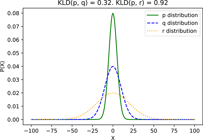
(a) p ≡ 𝒩(μ = 0, σ = 5), q ≡ 𝒩(μ = 0, σ = 10), r ≡ 𝒩(μ = 0, σ = 20)
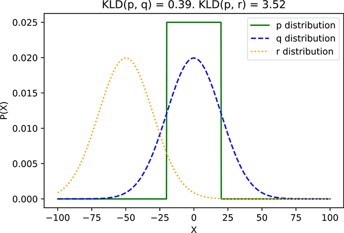
(b) p ≡ U(a = −20, b = 20), q ≡ 𝒩(μ = 0, σ = 20), r ≡ 𝒩(μ = −50, σ = 20)
Figure 6.4 KLD between example distributions
Similarly,
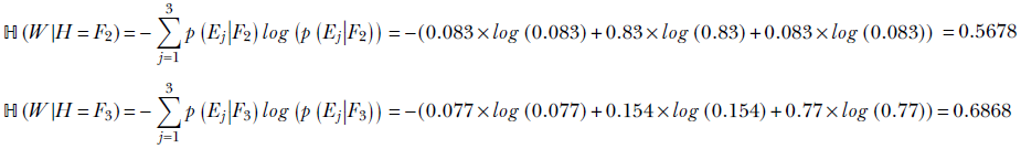
ℍ(W|H = Fi) is the entropy of W given H = Fi for i = 1 or 2 or 3. What is the overall conditional entropy of W given H: that is, ℍ(W|H)? To compute this, we take the expected value (that is, the probability-weighted average; see equation 5.8) of the conditional entropy ℍ(W|H = Fi) over all possible values of i:

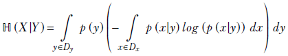
This idea can be generalized. Formally, given two random variables X and Y that can take values x ∈ Dx, ![]() ∈ Dy, respectively,
∈ Dy, respectively,
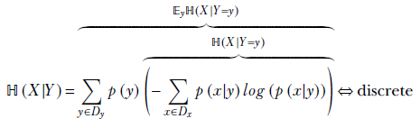
Equation 6.16
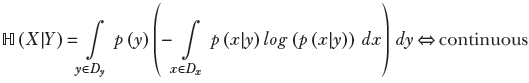
Equation 6.17
6.5.1 Chain rule of conditional entropy
ℍ(X|Y) = ℍ(X, Y) − ℍ(Y)
Equation 6.18
This can be derived from equation 6.17.
Applying Bayes’ theorem (equation 6.1),

Equation 6.19
6.6 Model parameter estimation
Suppose we have a set of sampled input data points X = {![]() (1),
(1), ![]() (2),⋯,
(2),⋯, ![]() (n)} from a distribution. We refer to the set collectively as training data. Note that we are not assuming it is labeled training data—we do not know the outputs corresponding to the inputs
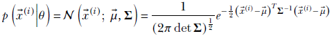
(n)} from a distribution. We refer to the set collectively as training data. Note that we are not assuming it is labeled training data—we do not know the outputs corresponding to the inputs ![]() (i). Also, suppose that based on our knowledge of the problem, we have decided which model family to use. Of course, simply knowing the family is not enough; we need to know (or estimate) the model parameters before we can use the model. For instance, our model family might be Gaussian, 𝒩(x;
(i). Also, suppose that based on our knowledge of the problem, we have decided which model family to use. Of course, simply knowing the family is not enough; we need to know (or estimate) the model parameters before we can use the model. For instance, our model family might be Gaussian, 𝒩(x; ![]() , Σ). Until we know the actual value of the parameters
, Σ). Until we know the actual value of the parameters ![]() and Σ, we do not fully know the model and cannot use it.
and Σ, we do not fully know the model and cannot use it.
How do we estimate the model parameters from the unlabeled training data? This is what we cover in this section. At the moment, we are discussing it without referring to any specific model architecture, so let’s denote model parameters with a generic symbol θ. For instance, when dealing with Gaussian models, θ = {![]() , Σ}.
, Σ}.
6.6.1 Likelihood, evidence, and posterior and prior probabilities
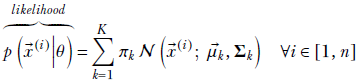
Before tackling the problem of parameter estimation, it is important to have a clear understanding of the terms likelihood, evidence, posterior probability, and prior probability in the current context. Equation 6.20 illustrates them. Using Bayes’ theorem,
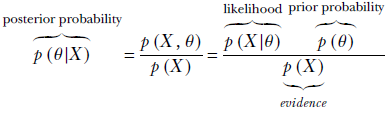
Equation 6.20
Let’s first examine the likelihood term. Using the fact that data instances are independent of each other,
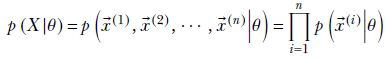
Now, p(![]() (i)|θ) is essentially the probability density of the distribution family we have chosen. For instance, if the model in question in Gaussian, then given θ = {
(i)|θ) is essentially the probability density of the distribution family we have chosen. For instance, if the model in question in Gaussian, then given θ = {![]() , Σ}, this will be
, Σ}, this will be
which is basically an expression for the Gaussian PDF: a restatement of equation 5.23 (but in equation 5.23, we dropped the “given θ,” part in the notation and expressed p(![]() |θ) simply as p(
|θ) simply as p(![]() )). Thus, we can always express the likelihood from the PDF of the chosen model family using the independence of individual training data instances.
)). Thus, we can always express the likelihood from the PDF of the chosen model family using the independence of individual training data instances.
Now let’s examine the prior probability, p(θ). It typically comes from some physical constraint—without referring to the input. A very popular approach is to say that, all other things being equal, we prefer parameters with smaller magnitudes. By this token, the larger the total magnitude ||θ||2, the lower the prior probability. For instance, we may use
p(θ) ∝ e−||θ||2
Equation 6.21
An indirect justification for favoring parameter vectors with the smallest length (magnitude) can be found in the principle of Occam’s razor. It states, Entia non sunt multiplicanda praeter necessitatem, which roughly translates to “One should not multiply unnecessarily.” This is often interpreted in machine learning and other disciplines as “favor the briefest representation.”
As shown previously, we can always express the likelihood and prior terms. Using them, we can formulate different paradigms, each with a different quantity, to optimize in order to estimate the unknown probability distribution parameters from training data. These techniques can be broadly classified into the following categories:
-
Maximum likelihood parameter estimation MLE)
-
Maximum a posteriori (MAP) parameter estimation
We provide an overview of them next. You will notice that, in all the methods, we typically preselect a distribution family as a model and then estimate the parameter values by maximizing one probability or another.
Later in the chapter, we look at MLE in the special case of the Gaussian family of distributions. Further down the line, we look at MLE with respect to Gaussian mixture models. Another technique outlined later is evidence maximization: we will visit it in the context of variational autoencoders.
6.6.2 Maximum likelihood parameter estimation (MLE)
In MLE of parameters, we ask, “What parameter values will maximize the joint likelihood of the training data instances?” In this context, remember that likelihood is the of a data instance occurring given specific parameter values (equation 6.20). Expressed mathematically,
MLE estimates what value of θ maximizes p(X|θ). The geometric mental picture is as follows: we want to estimate the unknown parameters for our model probability distribution such that if we draw many samples from that distribution, the sample point cloud will largely overlap the training data.
Often we employ the log-likelihood trick and maximize the log-likelihood instead of the actual likelihood.
For some models, such as Gaussians, this maximization problem can be solved analytically, and a closed-form solution can be obtained (as shown in section 6.8). For others, such as Gaussian mixture models (GMMs), the maximization problem ields no closed-form solution, and we go for an iterative solution (as shown in section 6.9.4).
6.6.3 Maximum a posteriori (MAP) parameter estimation and regularization
Instead of asking what parameter value maximizes the probability of occurrence of the training data instances, we can ask, “What are the most probable parameter values, given the training data?” Expressed mathematically, in MAP, we directly estimate the θ that maximizes p(θ|X). Using equation 6.20,
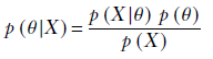
Equation 6.22
Since the denominator is independent of θ, maximizing the numerator with respect to θ maximizes the fraction. Thus
In MAP parameter estimation, we look for parameters θ that maximize p(X|θ)p(θ).
-
The first factor, p(X|θ), is what we optimized in MLE and comes from the model definition (such as equation 5.23 for multivariate Gaussian models).
-
The second factor, p(θ), is the prior term, which usually incentivizes the optimization system to choose a solution with predefined properties like smaller parameter magnitudes equation 6.21).
Viewed this way, MAP estimation is equivalent to MLE parameter estimation with regularization. Regularization is a technique often used in optimization. In regularized optimization, we add a term to the expression being maximized or minimized. This term effectively incentivizes the system to choose the solution with the smallest magnitudes of the unknown from the set of possible solutions. It is easy to see that MAP estimation essentially imposes the prior probability term on top of MLE. This extra term acts as a regularizer, incentivizing the system to choose the lowest magnitude parameters while still trying to maximize the likelihood of the training data.
Equation 6.22 can be interpreted another way. When we have no training data, all we can do is estimate the parameters from our prior beliefs about the system: the prior term p(θ). When the training data set X arrives, it influences the system through the likelihood term p(X|θ). As more and more training data arrives, the prior term (whose magnitude does not change with training data) dominates less and less, and the posterior probability p(θ|X) is dominated more by the likelihood.
6.7 Latent variables and evidence maximization
Suppose we have the height and weight data for a population (say, for the adult residents of our favorite town, Statsville). A single data instance looks like this:
Although the data is not explicitly labeled or classified, we know the data points can be clustered into two distinct classes, male and female. It is reasonable to expect that the distribution of each class is much simpler than the overall distribution. For instance, here, the distributions for males and females may be Gaussians individually (presumably, the means for females will occur at smaller height and weight values). The combined distribution does not fit any of the distributions we have discussed so far (later, we see it is a Gaussian mixture).
We look at such situations in more detail in connection to Gaussian mixture modeling and variational autoencoders. Here we only note that in these cases, it is often beneficial to introduce a variable for the class, say Z. In this example, Z is discrete: it can take one of two values, male or female. Then we can model the overall distribution as a combination of simple distributions, each corresponding to a specific value of Z.
Such variables Z that are not part of the observed data X but are introduced to facilitate modeling are called latent or hidden variables/parameters. Latent variables are connected to observed variables through the usual Bayesian expression:
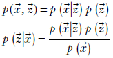
How do we estimate the distribution of Z? One way is to ask, “What distribution of the hidden variables would maximize the probability of exactly these training data points being returned if we drew random samples from the distribution?” The philosophy behind this is as follows: we assume that the training data points are fairly typical and have a high probability of occurrence in the unknown data distribution. Hence, we try to find a distribution under which the training data points will have the highest probabilities.
Geometrically speaking, each data point (vector) can be viewed as a point in some d-dimensional space, where d is the number of elements in the vector ![]() i. The training data points typically occupy a region within that space. We are looking for a distribution whose mass is largely aligned with the training data region. In other words, the probability associated with the training data points is as high as possible—the sample distribution cloud largely overlaps the training data cloud.
i. The training data points typically occupy a region within that space. We are looking for a distribution whose mass is largely aligned with the training data region. In other words, the probability associated with the training data points is as high as possible—the sample distribution cloud largely overlaps the training data cloud.
Expressed mathematically, we want to identify p(![]() |
|![]() ) and p(
) and p(![]() ) that maximize the quantity
) that maximize the quantity
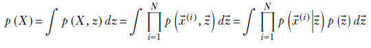
Equation 6.23
As usual, we get p(![]() (i)|
(i)|![]() ) from the PDF of our chosen model family and p(
) from the PDF of our chosen model family and p(![]() ) through some physical constraint.
) through some physical constraint.
6.8 Maximum likelihood parameter estimation for Gaussians
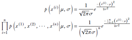
We look at this with a one-dimensional example, but the results derived apply to higher dimensions. Suppose we are trying to predict whether an adult Statsville resident is female, given that the resident’s height lies in a specified range [a, b]. For this purpose, we have collected a set of height samples of adult female Statsville residents. These height samples constitute our training data. Let’s denote them as x(1), x(2), ⋯, x(n). Based on physical considerations, we expect the distribution of heights of adult Statsville females to be a Gaussian distribution with unknown mean and variance. Our goal is to determine them from the training data via MLE, which effectively estimates a distribution whose sample cloud maximally matches the distribution of the training data points.
Let’s denote the (as yet unknown) mean and variance of the distribution as μ and σ. Then, from equation 5.22, we get
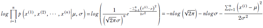
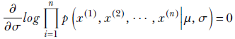
Employing the log-likelihood trick,
To maximize with respect to μ, we solve
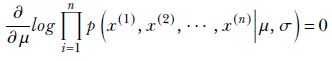
or
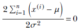
or
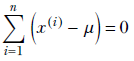
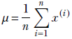
Finally, we get a closed-form expression for the unknown μ in terms of the training data:
Similarly, to maximize with respect to σ, we solve
or
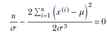
or
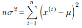
Finally, we get a closed-form expression for the unknown σ in terms of the training data:
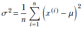
Thus we see that for a Gaussian, the maximum-likelihood solutions coincide with the sample mean and variance of the training data. Once we have the mean and standard deviation, we can calculate the probability that a female resident’s height belongs to a specified range [a, b] by using the following equation:

Equation 6.24
Given a training dataset, {![]() (1),
(1), ![]() (2),⋯,
(2),⋯, ![]() (n)}, the best fit Gaussian has the mean
(n)}, the best fit Gaussian has the mean

Equation 6.25
and the covariance matrix

Equation 6.26
We began this section by stating the problem of estimating the probability of an adult Statsville resident being female, given that their height lies in a specified range [a, b], when we are provided a training dataset of n height values of adult Statsville female residents. Let’s now revisit that problem. Using (scalar versions of) equations 6.25 and 6.26, we can estimate μ and σ and thereby define a Gaussian probability distribution
p(x) = 𝒩(x; μ, σ)
Using this, given any height x, we can compute the probability p(x) that the resident is female. Let’s see this using PyTorch.
6.8.1 Python PyTorch code for maximum likelihood estimation
Suppose we assume that the height values of adult female residents of Statsville follow a Gaussian distribution. If we know the parameters of this Gaussian (μ and σ), we know the Gaussian distribution fully. That allows us to estimate many interesting things: for instance, the expected height of an adult female resident of Statsville, or the probability that the height of an adult female Statsville resident lies in a certain range such as between 160 and 170 cm. The problem is, in a typical real-life situation, we do not know the parameters μ cm and σ. All we have is a large dataset X of height values of adult Statsville female residents—training data. We have to use this data to estimate the unknown parameters μ cm and σ. Once we have these, we have an estimated distribution (aka model) from which we can predict the probabilities of events of interest.
As we saw in section 6.6.2, MLE is a technique to estimate the parameters from given training data when the family to which the distribution belongs is known but the exact values of the parameters are not known. Listing 6.4 shows the PyTorch implementation of MLE for the Gaussian family.
NOTE Fully functional code for model parameter estimation using MLE and MAP, executable via Jupyter Notebook, can be found at http://mng.bz/9Mv7.
Listing 6.4 Maximum likelihood estimate for a Gaussian
sample_mean = X.mean()                          ①

sample_std = X.std()

gaussian_mle = Normal(sample_mean, sample_std)  ②

a, b = torch.Tensor([160]), torch.Tensor([170]) ③

prob = gaussian_mle.cdf(b) - gaussian_mle.cdf(a)
① Estimates Gaussian MLE parameters ![]() and Σ. They equal the sample mean and sample covariance of the training data. See equations 6.25 and 6.26.
and Σ. They equal the sample mean and sample covariance of the training data. See equations 6.25 and 6.26.
② Defines a Gaussian with the estimated parameters
③ Once the Gaussian is estimated, we can use it to predict probabilities.
6.8.2 Python PyTorch code for maximum likelihood estimation using gradient descent
In listing 6.4, we computed the MLE using the closed-form solution. Now, let’s try to compute the MLE using a different method: gradient descent. In real-life scenarios, we do not use gradient descent to compute the MLE because the closed-form solution is available. However, we discuss this method here to highlight some of the challenges of using gradient descent and how MAP estimation addresses these challenges.
Our goal is to maximize the likelihood function using gradient descent. This can alternatively be viewed as minimizing the negative log-likelihood function. We choose to use the logarithm of the likelihood function since that leads to simpler computation without any loss of generalization. (If you want a quick refresher on gradient descent, see section 3.5.) Following is the equation for negative log-likelihood:
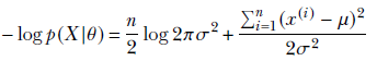
Equation 6.27
Listings 6.5 and 6.6 show the PyTorch code for the minimization process.
Listing 6.5 Gaussian negative log-likelihood for training data
def neg_log_likelihood(X, mu, sigma):                      ①
    N = X.shape[0]
    X_minus_mu = torch.sub(X, mu)
    t1 = torch.mul(0.5 * N,
               torch.log(2 * np.pi * torch.pow(sigma, 2))) ②

    t2 = torch.div(torch.matmul(X_minus_mu.T, X_minus_mu),
                 2 * torch.pow(sigma, 2))                  ③

    return t1 + t2                                         ④
① Equation 6.27
② n/2 log 2 πσ2
③ (Σi = 1n (xi – μ)2)/(2σ2)
④ Note how all the training data X is crunched in a single operation. Such vector operations are parallel and very efficient in PyTorch.
Listing 6.6 Minimizing MLE loss via gradient descent
def minimize(X, mu, sigma, loss_fn, num_iters=100, lr = 0.001): ①

    ②
   for i in range(num_iters):

        loss = loss_fn(X, mu, sigma)                            ③

        loss.backward()                                         ④

        mu.data -= lr * mu.grad
        sigma.data -= lr * sigma.grad                           ⑤

        mu.grad.data.zero_()
        sigma.grad.data.zero_()                                 ⑥

mu = Variable(torch.Tensor([5]).type(dtype), requires_grad=True)
sigma = Variable(torch.Tensor([5]).type(dtype), requires_grad=True)

minimize(X, mu, sigma, neg_log_likelihood)
① Negative log-likelihood (listing 6.5)
② Iterates to train
③ Computes the loss
④ Computes the gradients of the loss with regard to μ and σ. PyTorch stores the gradients in μ.grad and σ.grad.
⑤ Scales the gradients by learning the rate and update parameters
⑥ Resets the gradients to zero post-update
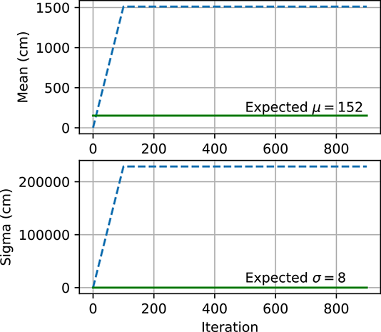
(a) MLE explodes: μinit = 1, σinit = 1.
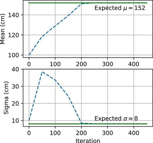
(b) MLE converges: μinit = 100, σinit = 10.
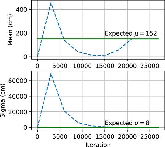
(c) MAP converges: μinit = 1, σinit = 1.
Figure 6.5 Gaussian parameter estimation using maximum likelihood estimate and maximum a posteriori estimation. In figure 6.5a, the MLE explodes because μ and σ are initialized far from μexpected and σexpected. However, the MLE converges in figure 6.5b because μ and σ are initialized closed to μexpected and σexpected. Figure 6.5c shows how, for MAP, μ and σ are able to converge to μ.expected and σexpected even though they are initialized far away.
Figure 6.5 shows how μ and σ change with each iteration of gradient descent. We expect μ and σ to end up close to μexpected and σexpected, respectively. However, when μ and σ start off far from μexpected and σexpected as in figure 6.5a), they do not converge to the expected values and instead become very large numbers. On the other hand, when they are instantiated with values closer to μexpected and σexpected as in figure 6.5b), they converge to the expected values. MLE is very sensitive to the initial values and has no mechanism to prevent the parameters from exploding. This is why MAP estimation is preferred. The prior p(θ) acts as a regularizer and prevents the parameters from becoming too large. Figure 6.5c shows how μ and σ converge to the expected values using MAP even though they started far away.
The MAP loss function is as follows. Note that it is the same equation as the negative log-likelihood, but with two additional terms—μ2 and σ2—that act as regularizers:
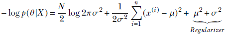
Equation 6.28
Listing 6.7 Gaussian negative log-likelihood with regularization
def neg_log_likelihood_reg(X, mu, sigma, k=0.2):               ①
    N = X.shape[0]
    X_minus_mu = torch.sub(X, mu)
    t1 = torch.mul(0.5 * N,
                   torch.log(2 * np.pi * torch.pow(sigma, 2))) ②

    t2 = torch.div(torch.matmul(X_minus_mu.T, X_minus_mu),
                   2 * torch.pow(sigma, 2))                     ③

    loss_likelihood = t1 + t2                                   ④

    loss_reg = k * (torch.pow(mu, 2) + torch.pow(sigma, 2))     ⑤

    return loss_likelihood + loss_reg                           ⑥
① Equation 6.28
② n/2 log 2 πσ2
③ (Σi = 1n (xi – μ)2)/(2σ2)
④ Negative log-likelihood
⑤ Regularization
⑥ Note how all the training data X is crunched in a single operation. Such vector operations are parallel and very efficient in PyTorch.
6.9 Gaussian mixture models
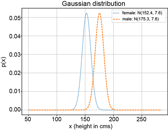
In many real-life problems, the simple unimodal (single-peak) probability distributions we learned about in chapter 5 fail to model the true underlying distribution of the data. For instance, consider a situation where we are given the heights of many adult Statsville residents. Say there are two classes of adults in Statsville: male and female. The height data we have is unlabeled, meaning we do not know whether a given instance of height data is associated with a male or a female. Thus the data is one-dimensional, and there are two classes. Figure 6.6 depicts the situation. None of the simple probability distributions we discussed in chapter 5 can be fitted to figure 6.6. But the two partial bells in figure 6.6a suggest that we should be able to mix a pair of Gaussians (each of which looks like a bell) to mimic this distribution. This is also consistent with our knowledge that the distribution represents not one but two classes, each of which can be reasonably represented individually by Gaussians. The point cloud also indicates two separate clusters of points. While a single Gaussian will not work, a mixture of two separate 1D Gaussians can (and, as we shall shortly see, will) work.
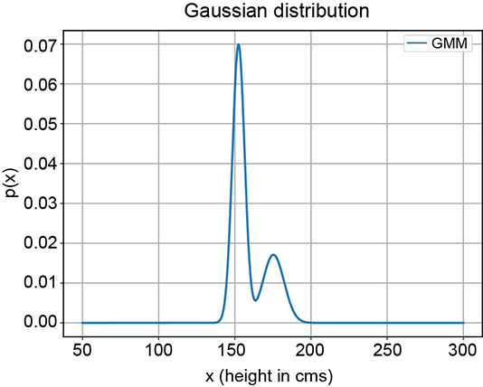
(a) PDF
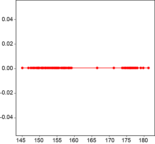
(b) Sample point distribution
Figure 6.6 Probability density functions (PDFs) and sample point distributions for 1D height data of adult male and female residents of Statsville
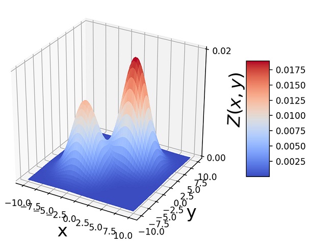
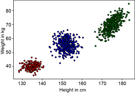
Let’s now discuss a slightly more complex problem in which the data is two-dimensional and has three classes. Here we are given the weights and heights of three classes of Statsville residents: adult females, adult males, and children. Again, the data is unlabeled, meaning we do not know whether a given instance of (height, weight) data is associated with a man, woman, or child. This is depicted in figure 6.7. Once again, none of the simple probability distributions we studied in chapter 5 can be fitted to this situation. But the PDF shows three bell-shaped peaks, the point cloud shows three clusters, and the physical nature of the problem indicates three separate classes, each of which can be reasonably represented by Gaussian. While a single Gaussian will not work, a mixture of three separate 2D Gaussians can (and, as we shall shortly see, will) work.
A Gaussian mixture model (GMM) is a weighted combination of a specific number of Gaussian components.
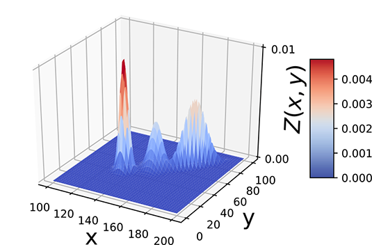
(a) PDF
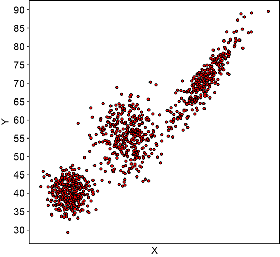
(b) Sample point distributions
Figure 6.7 Probability density functions (PDFs) and sample point distributions for 2D (height, weight) data of children, adult males, and adult females of Statsville
For instance, in our first problem with one dimension and two classes, we choose a mixture of two 1D Gaussians. For the second problem, we take a mixture of three 2D Gaussians. Each individual Gaussian component corresponds to a specific class.
6.9.1 Probability density function of the GMM
Formally,
The PDF for a GMM is
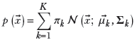
Equation 6.29
where πk is the weight of the kth Gaussian component, satisfying

K is the number of classes or Gaussian components, and 𝒩(![]() ;
; ![]() k, Σk) defined in equation 5.23) is the PDF for the kth Gaussian component. Such a GMM models a K-peaked PDF or, equivalently, a K-clustered sample point cloud.
k, Σk) defined in equation 5.23) is the PDF for the kth Gaussian component. Such a GMM models a K-peaked PDF or, equivalently, a K-clustered sample point cloud.
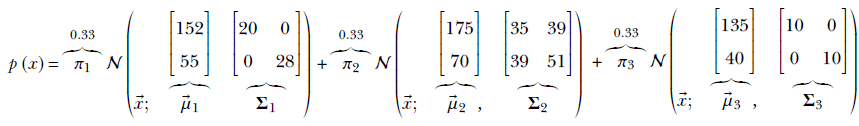
For instance, the PDF and sample point clouds shown in figure 6.6 correspond to the following Gaussian mixture:
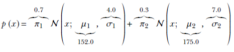
The 2D three-class problem, PDF, and sample point clouds shown in figure 6.7 correspond to the following Gaussian mixture:
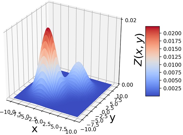
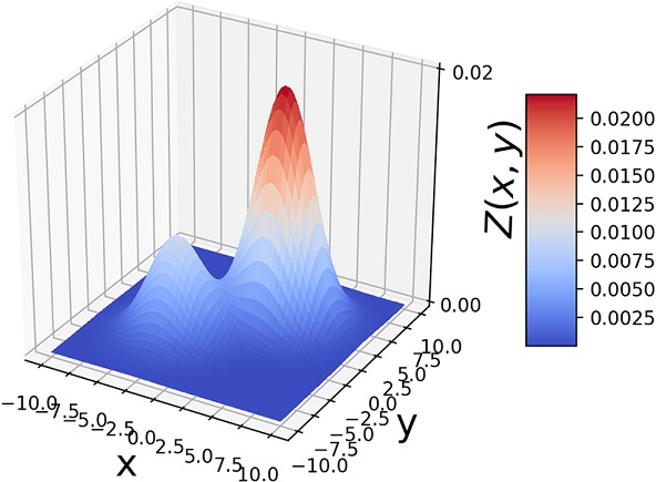
The PDF and sample point distribution of the GMM depend on the values of πks, μks, Σks, and K. In particular, K influences the number of peaks in the PDF (although if two peaks are very close, sometimes they merge). It also influences the number of clusters in the sample point cloud (again, if two clusters are too close, they may not be visually distinct). The πks regulate the relative heights of the hills. The μks and Σks influence the individual hills in the PDF as well as the individual clusters in the sample point cloud. Specifically, μk regulates the locations of the kth peak in the PDF and the centroid of the kth cluster in the sample point cloud. The Σks regulate the shape of the kth individual hill and the kth cluster in the sample point cloud. Figures 6.8, 6.9, 6.10, and 6.11 show some example GMMs with various values of these parameters.
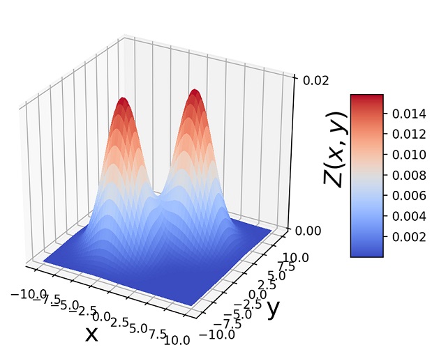
Figure 6.8 shows a pair of Gaussian distributions and various GMMs with those as components, with different values for the parameters. Figure 6.9 depicts 2D GMMs with various πks. Figure 6.10 shows GMMs with non-circular bases (non-symmetric Σs) and various μs).
(a) Gaussian components μ1 = 152, μ2 = 175, σ1 = σ2 = 9
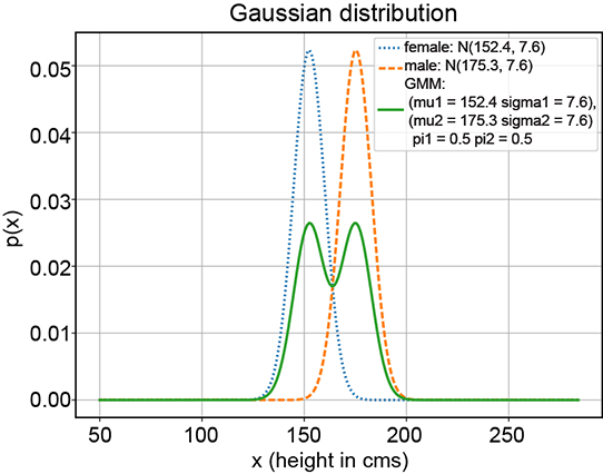
(b) GMM with π1 = 0.5, π2 = 0.5
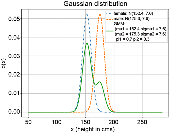
(c) GMM with π1 = 0.7, π2 = 0.3
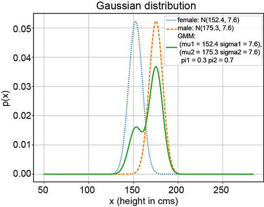
(d) GMM with π1 = 0.3, π2 = 0.7
Figure 6.8 Various GMMs (solid curves) with the same Gaussian components (dotted and dashed curves, respectively) but different π1 and π2 values
Another way to visualize GMMs is via sample point distributions. Figure 6.11 shows the sample points from a pair of 2D Gaussians and the points sampled from a GMM having those Gaussians as components and various mixture-selections probabilities.
(a) π1 = 0.5, π2 = 0.5
(b) π1 = 0.4, π2 = 0.6
(c) π1 = 0.7, π2 = 0.3
(d) π1 = 0.3, π2 = 0.7
Figure 6.9 Two-dimensional GMMs with circular bases,
 .
.
Note how the relative heights of the hills depend on πs.
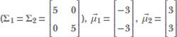
(a) ![]()
(b) ![]()
Figure 6.10 Two-dimensional GMMs with elliptical bases, π1 = 0.3, π2 = 0.7. Note how the shape of the hill base depends on Σ and how the hill positions depend on the ![]() s.
s.
(a)
(b)
Figure 6.11 (a)  . (b) 1, 000 random samples from a GMM with the same three component Gaussians as in (a) and π1 = π2 = 0.4, π3 = 0.2. Note how the GMM sample distribution shape mimics the combined sample distribution shape of the component Gaussians.
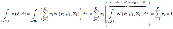
It can be proved that equation 6.29 is a proper probability: that is, it sums to 1 over the space of all possible inputs (all possible values of ![]() in the d-dimensional space). Here is the proof outline:
in the d-dimensional space). Here is the proof outline:
6.9.2 Latent variables for class selection
Let’s discuss GMMs in more detail. In particular, we look at the physical meaning of the various terms in equation 6.29.
Before diving in, let’s introduce an auxiliary random variable Z, which effectively is a class selector. In the context of equation 6.29, Z can take discrete values in the range [1⋯K]. It thus follows a categorical distribution (see section 5.9.6). Physically, Z = k means the kth class—that is, the kth component of the Gaussian mixture—has been selected.
NOTE As usual, we are denoting the random variable with uppercase and the specific value it takes in a given instance with lowercase.
For instance, in the two-class problem shown in figure 6.6, Z can take one of two values: 1 (implying adult female) or 2 (implying adult male). For the three-class problem shown in figure 6.7, Z can take one of three values: 1 (adult female), 2 (adult male), or 3 (child). Z is called a latent (hidden) random variable because its values are not directly observed. Contrast this with the input random variable ![]() whose values are explicitly observed. You may recognize Z as a latent variable in the GMM (latent variables were introduced in section 6.7).
whose values are explicitly observed. You may recognize Z as a latent variable in the GMM (latent variables were introduced in section 6.7).
Consider the joint probability p(X = ![]() , Z = k), which we sometimes informally denote as p(
, Z = k), which we sometimes informally denote as p(![]() , k). This is the probability of the input variable
, k). This is the probability of the input variable ![]() occurring together with the class k. Using Bayes’ theorem,
occurring together with the class k. Using Bayes’ theorem,
p(![]() , k) = p(
, k) = p(![]() |k)p(k)
|k)p(k)
The conditional probability term p(![]() |k) is the probability of
|k) is the probability of ![]() when the kth class has been selected. This means it is the PDF for the kth Gaussian component, which is a Gaussian distribution by assumption. As such, using equation 5.23,
when the kth class has been selected. This means it is the PDF for the kth Gaussian component, which is a Gaussian distribution by assumption. As such, using equation 5.23,
p(![]() |k) = 𝒩(
|k) = 𝒩(![]() ;
; ![]() k, Σk) k ∈ [1, K]
k, Σk) k ∈ [1, K]
On the other hand, p(Z = k), which we sometimes informally refer to as p(k), is the prior probability (that is, without reference to the input) of the input belonging to one of the classes. Let’s denote it as follows:
p(k) = πk, ∀k ∈ {1, K}
This is often modeled as the fraction of training data points belonging to class k:
![]()
where Nk is the number of training data instances belonging to class k, and N is the total number of training data instances.
From this, we get
p(![]() , k) = p(k)p(
, k) = p(k)p(![]() |k) = πk 𝒩(
|k) = πk 𝒩(![]() ;
; ![]() k, Σk) k ∈ [1, K]
k, Σk) k ∈ [1, K]
From equation 5.5, we get the marginal probability p(x)
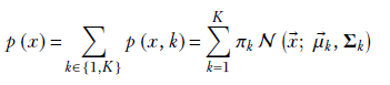
which is the same as equation 6.29.
This leads to the following physical interpretations:
-
A GMM can be viewed as a weighted sum of K Gaussian components. Equation 6.29 depicts the PDF of the overall GMM.
-
The weights πk are component selection probabilities. Specifically, πk can be interpreted as the prior probability p(Z = k), aka p(k), of selecting the kth subclass—modeled as the fraction of the population belonging to the kth subclass. The πk are probabilities in a categorical distribution with K classes. The πks sum up to 1. Sampling from the GMM can be viewed as a two-step process:
-
Randomly select a component. The probability of the kth component being selected is πk. The sum of all πks is 1, which signifies that one or another component must be selected.
-
Random sample from the selected Gaussian component. The probability of generating vector
 is 𝒩(;
  k, Σk).
-
-
Each of the K Gaussian components models an individual class. Geometrically speaking, the components correspond to the clusters in the sample point cloud or the peaks in the PDF of the GMM.
-
The kth Gaussian component, 𝒩(
; k, Σk), can be interpreted as the conditional probability, p(|k). This is the likelihood—the probability of data value occurring, given that the kth subclass has been selected. -
The product πk 𝒩(
; k, Σk) then represents the joint probability p(, k) = p(|k) p(k). -
The sum of all the joint subclass probabilities is the marginal probability p(
) of the data value .
Listing 6.8 Gaussian mixture model distribution
from torch.distributions.mixture_same_family import MixtureSameFamily ①

pi = Categorical(torch.tensor([0.4, 0.4, 0.2]))                       ②

mu = torch.tensor([[175.0, 70.0], [152.0, 55.0], [135.0, 40.0]])      ③

sigma = torch.tensor([[[30.0, 20.0], [20.0, 30.0]],                   ④
                     [[50.0, 0.0], [0.0, 10.0]],
                     [[20.0, 0.0], [0.0, 20.0]]])

gaussian_components = MultivariateNormal(mu, sigma)                   ⑤

gmm = MixtureSameFamily(pi, gaussian_components)                      ⑥
① Pytorch supports distributions that are mixtures of the same family (here, Gaussian)
② Prior probabilities over the three classes (male, female, child): categorical distribution
③ Mean height, weight for the three classes (male, female, child)
④ Covariance matrices for the three classes male, female, child)
⑤ Creates the component Gaussians
⑥ Creates the GMM
6.9.3 Classification via GMM
A typical practical problem involving GMMs goes as follows. A set of unlabeled input data X training data) is provided. It is important to note that this is unsupervised machine learning—the training data does not come with known output classes. The physical nature of the problem indicates the subclasses in the data (denoted by indices [1⋯K]). The goal is to classify any arbitrary input ![]() : that is, map it to one of the K classes. To do this, we have to fit a GMM (that is, derive the values of πk,
: that is, map it to one of the K classes. To do this, we have to fit a GMM (that is, derive the values of πk, ![]() k, Σk for all k ∈ [1 ⋯ K]). Given an arbitrary
k, Σk for all k ∈ [1 ⋯ K]). Given an arbitrary ![]() , we compute p(k|
, we compute p(k|![]() ) for all the classes (all values of k). The value of k yielding the max value for p(k|
) for all the classes (all values of k). The value of k yielding the max value for p(k|![]() ) is the class corresponding to
) is the class corresponding to ![]() . How do we compute p(k|
. How do we compute p(k|![]() )?
)?
Using Bayes’ theorem,
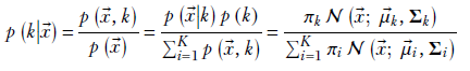
Equation 6.30
If we know all the GMM parameters, evaluating equation 6.30 is straightforward. We classify the input ![]() by assigning it to the cluster k that yields the highest value of p(Z = k|X = x). Geometrically, this assigns the input to the cluster with the “closest” mean—with distance normalized by the variance of the respective distribution. Basically, we are measuring the distance from the mean, but in clusters of high variance, we are more tolerant of distance from the mean. This makes intuitive sense: if the cluster is widely spread has high variance), a point relatively far from the cluster mean can be said to belong to the cluster. On the other hand, a point the same distance from the mean of a tightly packed cluster may be deemed to be outside the cluster.
by assigning it to the cluster k that yields the highest value of p(Z = k|X = x). Geometrically, this assigns the input to the cluster with the “closest” mean—with distance normalized by the variance of the respective distribution. Basically, we are measuring the distance from the mean, but in clusters of high variance, we are more tolerant of distance from the mean. This makes intuitive sense: if the cluster is widely spread has high variance), a point relatively far from the cluster mean can be said to belong to the cluster. On the other hand, a point the same distance from the mean of a tightly packed cluster may be deemed to be outside the cluster.
6.9.4 Maximum likelihood estimation of GMM parameters (GMM fit)
A GMM is fully described in terms of its parameter set θ = {πk, ![]() k, Σk ∀k ∈ [1 ⋯ K]}. But how do we estimate these parameter values? In typical real-life situations, they are not given to us. We only have a set of observed unlabeled training data points X = {
k, Σk ∀k ∈ [1 ⋯ K]}. But how do we estimate these parameter values? In typical real-life situations, they are not given to us. We only have a set of observed unlabeled training data points X = {![]() (i)}, such as (weight, height) values for Statsville residents.
(i)}, such as (weight, height) values for Statsville residents.
Geometrically speaking, each data instance in the training dataset corresponds to a single point in the multidimensional feature space. The training dataset is a point cloud that naturally clusters into Gaussian subclouds (otherwise, we should not be trying GMMs). Our GMM mimicking this dataset should have as many components as there are natural clusters in the data. The parameter values πk, ![]() k, Σk for k ∈ [1 ⋯ K] should be estimated such that the GMM’s sample point cloud overlaps the training data point cloud as much as possible. That is the basic problem we try to solve in this section.
k, Σk for k ∈ [1 ⋯ K] should be estimated such that the GMM’s sample point cloud overlaps the training data point cloud as much as possible. That is the basic problem we try to solve in this section.
NOTE We do not estimate K, the number of classes; rather, we use a fixed value of K, usually estimated from the physical conditions of the problem. For example, in the problem with men, women, and children, it is pretty obvious that K = 3.
In section 6.8, we did MLE for a simple Gaussian. We computed an expression for the joint log-likelihood of all the training data given a Gaussian probability distribution. Then we took the gradient of that expression with respect to the parameters and equated it to zero. We were able to solve that equation to derive a closed-form solution for the parameters, ![]() and Σ (equations 6.25 and 6.26 ). This means we simplified the equation into a form where the unknown (to be solved) appeared alone on the left-hand side and there were only known entities on the right-hand side.
and Σ (equations 6.25 and 6.26 ). This means we simplified the equation into a form where the unknown (to be solved) appeared alone on the left-hand side and there were only known entities on the right-hand side.
Unfortunately, with GMMs, equating the gradient of the log-likelihood to zero leads to an equation that has no closed-form solution. So, we cannot reduce the equation to a form where the unknowns πks, μks, and Σk appear alone on the left-hand sides and only known entities (![]() is) appear on the right-hand side. Consequently, we have to go for an iterative approximation. We rewrite the equation we get by equating the gradient of the log-likelihood to zero such that the unknowns μs and σs appear alone on the right-hand side. It looks something like
is) appear on the right-hand side. Consequently, we have to go for an iterative approximation. We rewrite the equation we get by equating the gradient of the log-likelihood to zero such that the unknowns μs and σs appear alone on the right-hand side. It looks something like
πk = f1(X, Θ)
![]() k = f2(X, Θ)
k = f2(X, Θ)
Σk = f3(X, Θ)
where f1, f2, f3 are some functions whose exact nature is unimportant at the moment. Note that the right-hand side also contains the unknowns: θ contains πks, μks, and Σk. We cannot directly solve such equations, but we can use iterative relaxation, which works roughly as follows:
-
Start with random values of πks,
ks, and Σks. -
Evaluate the right-hand side by plugging current values of πks,
ks, and Σks into functions f1, f2, and f3. -
Use the values estimated in step 2 to set new values of πks,
ks, and Σks. -
Repeat steps 1–3 until the parameter values stop changing appreciably.
The actual functions f1, f2, f3 are worked out in equations 6.36, 6.37, and 6.38). As iteration progresses, the values of πks, ![]() ks, and Σks start to converge to their true values. This is not a lucky coincidence. If we follow algorithm 6.3, it can be proved that every iteration improves the approximation, even if by a minuscule amount. Eventually, we reach a point when the approximation is no longer improving appreciably. This is called the fixed point, and we should stop iterating and declare the current values final.
ks, and Σks start to converge to their true values. This is not a lucky coincidence. If we follow algorithm 6.3, it can be proved that every iteration improves the approximation, even if by a minuscule amount. Eventually, we reach a point when the approximation is no longer improving appreciably. This is called the fixed point, and we should stop iterating and declare the current values final.
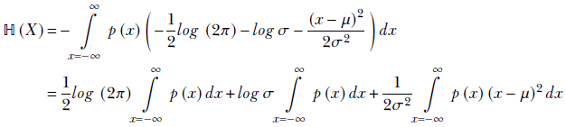
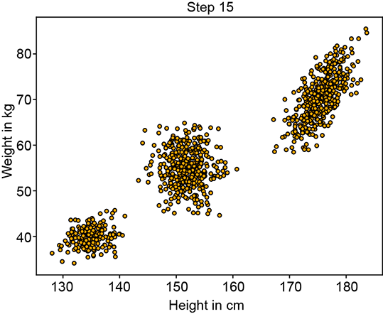
Figure 6.12 shows the progression of an iterative GMM fit algorithm. Figure 6.12a shows the sampled training data distribution. Figure 6.12b shows the fitted GMM at the beginning: the parameters are essentially random, and the GMM looks nothing like the target training data distribution. It improves slowly until at iteration 15, it matches the target distribution snugly figure 6.12d).
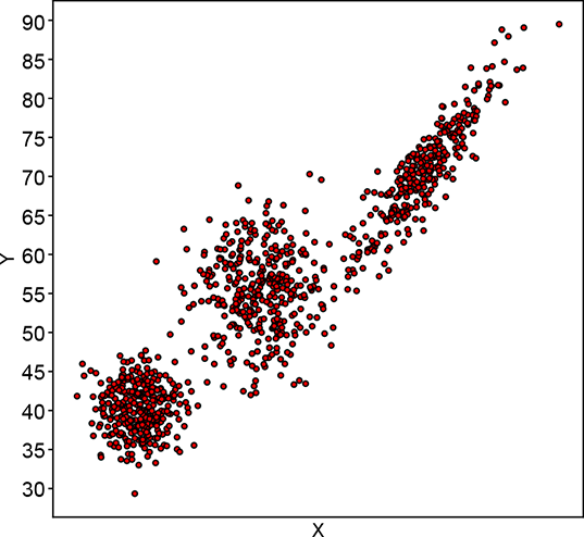
(a) Training data point cloud (target for fitting)
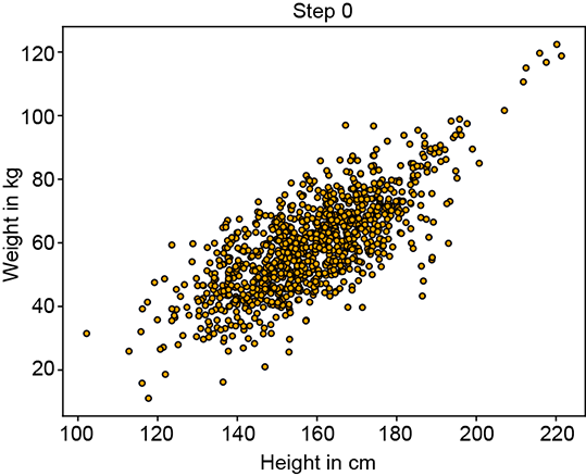
(b) Fitted GMM’s sample point cloud at step 0
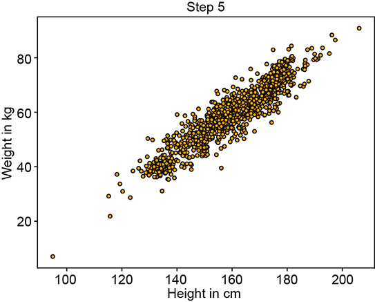
(c) Fitted GMM’s sample point cloud at step 5
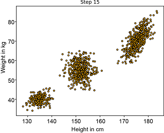
(d) Fitted GMM’s sample point cloud at step 15. It almost matches the target.
Figure 6.12 Progression of maximum likelihood estimation for GMM parameters
Now let’s discuss the details. We already know the dataset X that has been observed. What parameter set θ will maximize the conditional probability, p(X|θ), of exactly these data points, given the parameter set? In other words, what model parameters will maximize the overall likelihood of the training data? Those will be our best guesses for the unknown model parameters. This is MLE, which we encountered in section 6.6.2.
Let {![]() (1),
(1), ![]() (n),⋯
(n),⋯![]() (n)} be the set of observed data points, aka training data. From equation 6.29,
(n)} be the set of observed data points, aka training data. From equation 6.29,
Henceforth, for simplicity, we drop the “given θ” part and refer to p(![]() (i)|θ) simply as p(
(i)|θ) simply as p(![]() (i)). As usual, instead of maximizing the likelihood directly, we maximize its logarithm, the log-likelihood. This will yield the same parameters as maximizing the likelihood directly.
(i)). As usual, instead of maximizing the likelihood directly, we maximize its logarithm, the log-likelihood. This will yield the same parameters as maximizing the likelihood directly.
Since the x(i)s are independent, their joint probability, as per equation 5.4, is
p(![]() (1))p(
(1))p(![]() (2))⋯p(
(2))⋯p(![]() (n))
(n))
The corresponding log joint probability is
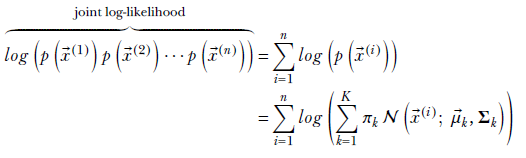
Equation 6.31
At this point, we begin to see a difficulty peculiar to GMMs. We have a logarithm of a sum, which is not a very friendly expression to handle; the logarithm of products is much nicer to deal with. But let’s soldier on.
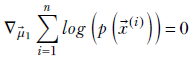
To identify the parameters ![]() 1, Σ1,
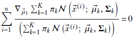
1, Σ1, ![]() 2, Σ2, ⋯ that will maximize the log joint probability, we take the gradient of the log joint probability with respect to these parameters, equate them to zero, and solve for the parameter value (as discussed in section 3.3.1). Here we demonstrate the process with respect to
2, Σ2, ⋯ that will maximize the log joint probability, we take the gradient of the log joint probability with respect to these parameters, equate them to zero, and solve for the parameter value (as discussed in section 3.3.1). Here we demonstrate the process with respect to ![]() 1:
1:
∇![]() 1log(p(
1log(p(![]() (1))p(
(1))p(![]() (2))⋯p(
(2))⋯p(![]() (n))) = 0
(n))) = 0
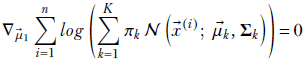
Since the log of products is the sum of logs, we get
Applying equation 6.29, we get
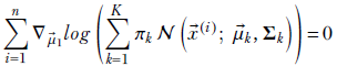
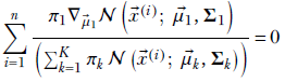
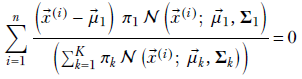
Since the gradient is a linear operator, we can move it inside the summation:
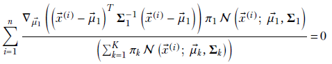
Since d/dx log (f(x)) = 1/f(x) df/dx, we get
Now, if x1 and x2 are independent variables, dx2/dx1 = 0. Consequently,
![]()
Only a single term corresponding to k = 1 survives the differentiation (gradient) in the numerator. So,
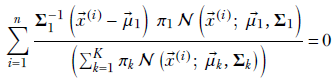
Now d/dx e–(x – μ)2 = –2(x – μ) e–(x – μ)2, and in multiple dimensions,
![]()
Plugging equation 5.23 into our maximization problem, we get
Furthermore, with a little effort, you can prove the following about the gradient of a quadratic form:
∇![]() (
(![]() TA
TA![]() ) = A
) = A![]()
Equation 6.32
Applying equation 6.32 to our problem, we get
Multiplying both sides by the constant Σ1, we get
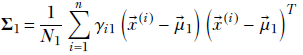
Substituting
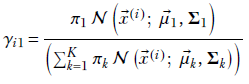
Equation 6.33
we get
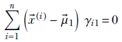
This expression has μ1 inside γi1 as well. It is impossible to extract μ1 alone on the left side of the equation. In other words, we cannot create a closed-form solution for μ1. Hence, we have to solve it iteratively.
We can rewrite the previous equation as
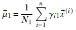
where

Equation 6.34
Proceeding similarly, we can derive the corresponding expressions for π1 and Σ1. Let’s collect all the equations for updating the GMM parameters:

Equation 6.35

Equation 6.36
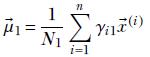
Equation 6.37
Equation 6.38
Equations 6.36, 6.37, and 6.38 provide the definitions for functions f1, f2, and f3 that we saw at the beginning of this section in the context of iterative relaxation. We can deal similarly with k = 2⋯K.
γik = p(k|![]() (i))
(i))
This gives us a new way to look at equations 6.35, 6.36, 6.37, and 6.38:
-
Equation 6.35 essentially assigns to N1 the probability mass concentrated in class 1 as per the current parameter values.
-
Equation 6.36 assigns to π1 the fractional mass in class 1 as per the current parameter values.
-
Equation 6.37 assigns to μ1 the centroid of all the training data points. Each data point’s contribution is weighted by the posterior probability, as per the current parameter values, of that data point belonging to class 1.
-
Equation 6.38 assigns to Σ1 the covariance of the training data points. Each data point’s contribution is weighted by the posterior probability, as per the current parameter values, of that data point belonging to class 1.
Algorithm 6.3 ties together equations 6.33, 6.36, 6.37, and 6.38 into a complete approach for iterative MLE of GMM parameters. It is an example of a general class of algorithms called expectation maximization.
Algorithm 6.3 GMM fit (MLE of GMM parameters from unlabeled training data)
Input: X = ![]() (1),
(1), ![]() (2), … ,
(2), … , ![]() (n)
(n)
Initialize parameters Θ = {πk , μk , Σk k ∈ [1, K]} with random values
⊳ repeat E-step and M-step until likelihood stops increasing
while (likelihood is increasing ) do
⊳E-step
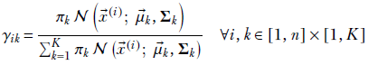
⊳M-step
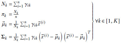
end while
return {x1 , μ1, Σ1, x2, μ2, Σ2 , … , xK, μK, ΣK}
NOTE Fully functional code for Gaussian mixture modeling, executable via Jupyter Notebook, can be found at http://mng.bz/j4er.
Listing 6.9 GMM fit
while (curr_likelihood - prev_likelihood) < 1e-4:     ①

  # E Step                                            ②

  pi = gmm.mixture_distribution.probs                 ③

  components = gmm.component_distribution             ④

   ⑤
   log_gamma_numerators = components.log_prob(
       X.unsqueeze(1)) + torch.log(pi).repeat(n, 1)   ⑥

   ⑦
   log_gamma_denominators = torch.logsumexp(
       log_gamma_numerators, dim=1, keepdim=True).

   ⑧
   log_gamma = log_gamma_numerators - log_gamma_denominators
   self.gamma = torch.exp(log_gamma)

   # M Step                                           ⑨

   n = X.shape[0]                                     ⑩

   N = torch.sum(gamma, 0)

   pi = N / n                                         ⑪

   mu = ((X.T @ gamma)/N).T                           ⑫

   x_minus_mu = (X.repeat(K, 1, 1) - gmm.component_distribution.unsqueeze(1).
                 repeat(1, n, 1))

   ⑬
   x_minus_mu_squared = x_minus_mu.unsqueeze(3)  @ x_minus_mu.unsqueeze(2)

   ⑭
   sigma = torch.sum(gamma.T.unsqueeze(2).unsqueeze(3) * x_minus_mu_squared,
                     axis=1) / N.unsqueeze(1).unsqueeze(1).repeat(1, d, d)

   prev_likelihood = curr_likelihood

   curr_likelihood = torch.sum(gmm.log_prob(X))       ⑮
① Repeats until the likelihood increase is negligible
② Computes the posterior probabilities γi,k = p(Z = k|X = xi) using current ![]() ks and Σks, equation 6.33
ks and Σks, equation 6.33
③ Tensor of shape [K] holding πks for all k
④ Gaussian objects 𝒩(![]() ,
, ![]() k, Σk) for all k
k, Σk) for all k
⑤ Vector computation of log of γi, k numerators for all i, k, equation 6.33
⑥ In practice, the probability involving an exponential goes to 0. So we use the log probability.
⑦ Vector computation of the log of γi, k denominators for all i, k, equation 6.33
⑧ Vector computation of the [n × K] tensor γi, k, equation 6.33
⑨ Updates ![]() k and Σk for all k using γi, k = p(Z = k|X) from the E-step via equations 6.36, 6.37, and 6.38
k and Σk for all k using γi, k = p(Z = k|X) from the E-step via equations 6.36, 6.37, and 6.38
⑩ Number of data points
⑪ Vector update of πk for all k, equation 6.36
⑫ Vector update of [K × d] tensor, ![]() k for all k, equation 6.37
k for all k, equation 6.37
⑬ Vector computation of (![]() i –
i – ![]() k) (
k) (![]() i –
i – ![]() k)T for all l, k
k)T for all l, k
⑭ Vector update of K × d × d] tensor Σk for all k, equation 6.38
⑮ log likelihood, equation 6.31
Summary
In this chapter, we looked at the Bayesian tools for decision-making in uncertain systems. We discussed conditional probability and Bayes’ theorem, which connects conditional probabilities to joint and marginal probabilities.
-
Conditional probability is the probability of an event occurring subject to the condition that another event has already occurred. In machine learning, we are often interested in the conditional probability p(
|θ) of an input given that the parameters of the model predicting the input are θ. This conditional probability is known as the likelihood of the input. We are also interested in the conditional probability p(θ|), known as the posterior probability. -
Joint probability is the probability of a set of events occurring together. If the events are independent, the joint probability is the product of their individual probabilities. Whether events are independent or not, Bayes’ theorem connects joint and conditional probabilities. Of particular interest in machine learning is the Bayes’ theorem expression connecting the likelihood and joint and posterior probabilities of inputs and parameters: p(
, θ) = p(|θ)p(θ) and p(|θ)p(θ) / p(). p(|θ) is the probability distribution function of the chosen distribution family. p(θ) is the prior probability that codifies our belief, sans data, about the system. A popular choice is p(θ) ∝ e−||θ||2, implying smaller probabilities for higher-magnitude parameters and vice versa. -
Entropy models the uncertainty in a system. Systems where all events have more or less similar probabilities tend to be high-entropy. Systems where a particular subset of possible events have significantly high probabilities and others have significantly low probabilities tend to be low-entropy. Equivalently, the probability density functions of low-entropy systems tend to have tall peaks, and their sample point clouds have a high concentration of points in some regions. High-entropy systems tend to have flat probability density functions and diffused sample point clouds.
-
Cross-entropy allows us to quantify how good our modeling is against a known ground truth.
-
Kullback–Leibler divergence gives us a measure of the dissimilarity between two probability distributions.
-
Maximum likelihood estimation (MLE) and maximum a posteriori (MAP) estimation are two paradigms for estimating model parameters. MLE maximizes p(X|θ), and MAP maximizes p(X|θ)p(θ). MLE essentially tries to estimate probability distribution parameters that maximize the overlap between the sample point cloud of the probability distribution and the training data point cloud. MAP is MLE with a regularization condition. The regularization condition is injected via the prior probability term p(θ), which favors solutions with a certain property (such as small parameter magnitudes) that we believe to be true from empirical knowledge without data. MLE for Gaussian distributions has a closed-form solution. The mean and variance (covariance in the multidimensional case) of the optimal probability distribution that best fits the training data are the sample mean and sample variance or covariance on the training dataset.
-
Latent variables in a machine learning system are auxiliary variables that are not directly observed but can be derived from the input. They facilitate the expression of the goal of optimization or the loss to be minimized.
-
Gaussian mixture models (GMM) are unsupervised probability models that fit multiclass data distributions having multiple clusters in the training dataset, each corresponding to a different class. Here, MLE does not yield a closed-form solution but instead yields an iterative solution to estimate the mixture weights, means, and variances of the individual Gaussians in the mixture.