7 Function approximation: How neural networks model the world
This chapter covers
- Expressing real-world problems as mathematical functions
- Understanding the building blocks of a neural network
- Approximating functions via neural networks
Computing to date has been dominated by the von Neumann architecture in which the processor and the program are separate. The program sits in memory and is fetched and executed by the processor. The advantage of this approach is that different programs solving unrelated problems can be loaded into memory, and the same processor can execute them. But neural networks have a fundamentally different architecture. There are no separate processors and programs; instead, there is a single entity called, well, the neural network, which can run on dedicated hardware or a Von Neumann computer. In this chapter, we discuss this paradigm in detail.
NOTE The complete PyTorch code for this chapter is available at http://mng.bz/K4zj in the form of fully functional and executable Jupyter notebooks.
7.1 Neural networks: A 10,000-foot view
In section 1.7, we provided an overview of neural networks. (You may want to do a quick refresher on chapter 1 at this point.) There we indicated that most intelligent tasks performed by humans can be expressed in terms of mathematical functions that we will refer to as target functions. So, to develop machines that perform intelligent tasks, we need to have machines that model target functions. While that gives us hope of developing automated solutions, we are hobbled by two serious difficulties:
-
In addition to being arbitrarily complicated, the target functions underlying various real-life problems are completely different from one another. There is hardly any common pattern.
-
For most problems, we do not know the underlying target function.
Despite all this, we want to come up with a mechanized repeatable solution for performing real-life intelligent tasks. And we do not want to start from scratch and design the underlying function for each such problem. This is where neural networks help:
Neural networks provide a unified framework to model an extremely wide variety of arbitrarily complicated functions.
While the overall neural network models a complicated function, its building block is a fairly basic unit called a neuron. The neuron represents a relatively simple function. The full neural network is made up of many neurons with weighted connections between them. It can be made to approximate any arbitrary target function underlying a particular problem of interest by manipulating the number of neurons, the connectivity between them, and the connection weights.
The variety and complexity of the functions a neural network can represent are known as its expressive power. Expressive power increases with the number of neurons in the neural network and the number of connections between them. The more complex the target function, the more expressive power will be needed in the neural network modeling it. How can we make a neural network model/approximate/express a specific target function corresponding to a particular problem of interest? Answer: we can adjust the following two aspects of the neural network:
-
Architecture—The number of neurons and the connections between them
-
Parameter values—The weights of the connection between neurons
The architecture is typically chosen based on the nature of the problem. Some popular architectures are reused frequently, and a neural network engineer typically chooses an architecture that is historically known to be effective for a problem similar to the problem at hand. We look at several popular architectures later in this book—for instance, in chapter 11. Once the architecture is set, we determine the parameter values through a process called training.
Neural networks can be classified into two major classes: supervised and unsupervised. In supervised neural networks, we identify the desired output values corresponding to a set of sampled input values for the problem we are trying to solve. The desired output for these sampled inputs is typically chosen manually using a process called labeling (aka manual annotation or manual curation). The overall set of <sampled input, desired output> pairs constitutes the supervised training data. The set of desired outputs for training data inputs is sometimes collectively referred to as the ground truth or target output.
During training, the parameter values (aka weights) are adjusted such that the network’s outputs on training inputs match the corresponding ground truth as closely as possible. If all goes well, at the end of training, we are left with a neural network whose outputs on training inputs are close to the ground truth. This trained neural network is then deployed to the real world, where it performs inferencing—it generates output on inputs it has never seen before. If we have chosen the architecture with enough expressive power and properly trained the network with adequate training data, it should emit accurate results during inferencing. Note that we cannot guarantee correct results during inferencing; we can only make a probabilistic statement that our output has a p probability of being correct.
Unsupervised neural networks do not need the manually labeled ground truth—they just work on the training inputs. The manual labor involved in labeling the training data is expensive and bothersome. Consequently, considerable research effort is going into neural networks that are unsupervised, semi-supervised (a fraction of the training data is labeled manually), or self-supervised (labeled training data is created programmatically rather than manually). However, unsupervised and semi-supervised neural network technology is less mature at the time of this writing, and it is harder to achieve desired accuracy levels with them. Later in this book, we examine unsupervised approaches, including variational autoencoders (chapter 14). But for now, we mostly talk about supervised approaches.
It is important to note that nowhere in the architecture selection or training process do we need a closed-form representation of either the function being approximated (the target function) or the approximator function (the modeling function). This is important. In most cases, it is impossible to know the target function—all we know are sample input and ground-truth pairs (training data). As for the modeling function, even when we know the architecture of the modeling neural network, the overall function it represents is so complicated that it is virtually intractable. Thus, the fact that we do not need to know the target or modeling function in closed form is what makes the technology practical.
7.2 Expressing real-world problems: Target functions
Consider the classic investor’s problem: to sell or not sell a stock. The problem inputs could be the purchase price, current price, whether the investor’s favorite expert is advising to sell or not, and so on. The problem can be solved by a function that takes these inputs and outputs as 0 (do not sell) or 1 (sell). If we could model this function, we would have a mechanical solution to this real-world problem.
Like this example, most real-world problems can be expressed as target functions. We collect all quantifiable variables that can have a bearing on the outcome: these constitute the input variables. The input variables are expressed as numeric entities: scalars, vectors, matrices, and so on. The outputs are also expressed as numeric variables called the output variables. Given a specific input (say, specific values for purchase price and current price), our model function emits an output (0 or 1 indicating do not sell or sell) that is a solution to the problem for that specific input.
We usually denote input variables with the symbol x; a sequence of input variables is often expressed as a vector ![]() . Output variables are denoted with the symbol y. The overall target function is usually expressed as y = f(
. Output variables are denoted with the symbol y. The overall target function is usually expressed as y = f(![]() ). We will often use subscripts to denote various elements of a vector (x0, x1, ⋯, xi) and superscripts to denote input instances, as in y(0) = f(
). We will often use subscripts to denote various elements of a vector (x0, x1, ⋯, xi) and superscripts to denote input instances, as in y(0) = f(![]() (0)), y(1) = f(
(0)), y(1) = f(![]() (1)), ⋯, y(i) = f(
(1)), ⋯, y(i) = f(![]() (i)). But in some cases, we will use subscripts to denote different items of the training data. The usage should be obvious from the context.
(i)). But in some cases, we will use subscripts to denote different items of the training data. The usage should be obvious from the context.
Numeric quantities can occur in two distinct forms: continuous and categorical. Continuous variables can take any of the infinitely many real number values in a given range. For instance, the stock price in our “to sell or not sell a stock” problem can take any value greater than zero. Categorical variables can take one of a finite set of allowed values, where the value represents a category. A special categorical case is a binary variable, where there are only two categories. For instance, expert advice in our stock-selling problem can take only two values: 0 or 1, corresponding to the two categories of advice, “do not sell” and “sell,” respectively.
In this section, we discuss three distinct families of target functions: logical functions, general functions, and classifiers.
7.2.1 Logical functions in real-world problems
These are functions whose inputs and outputs are binary variables: variables that can take only two values, 0 (aka “no” or “don’t fire”) and 1 (aka “yes” or “fire”). Machines emulating logical functions are often added on top of separate machines performing other tasks, as will be evident from the following examples:
-
Logical OR—To look at logical OR functions, let’s bring back the mythical cat whose brain we discussed in chapter 1. Say we are trying to build a machine that helps the poor creature make the binary decision whether to run away from the object in front of it or approach the object and purr. Being very timid, this cat runs away from anything that looks hard or sharp. The only time it will approach and purr is when the object in front of it looks neither hard nor sharp. Let’s assume a separate machine outputs a binary decision 0 not hard) or 1 (hard). Another machine outputs a binary decision 0 (not sharp) or 1 (sharp). The logical OR machine combines the binary decisions from the two separate machines, as shown in figure 7.1a.
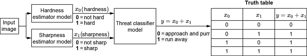
(a) Logical OR: a timid cat that runs away from things whose hardness exceeds threshold t0 OR whose sharpness exceeds threshold t1
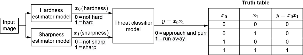
(b) Logical AND: a less timid cat that runs away from things whose hardness exceeds threshold t0 AND whose sharpness exceeds threshold t1
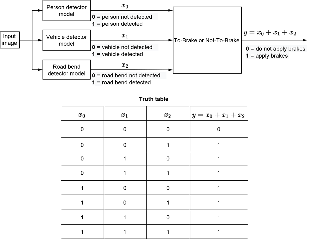
(c) Multi-input logical OR: A self-driving car that applies the brake if it sees a person, vehicle, or bend in the road in front of it
Figure 7.1 Examples of logical operators (OR, AND) in real-life problems
-
Logical AND—We also exemplify this in terms of the cat brain. Imagine a slightly less timid cat that runs away from things that are both hard and sharp. But it is not scared by hardness and sharpness alone. Its brain can be modeled by the system of machines shown in figure 7.1b.
-
Logical NOT—Consider a machine that sounds an alarm if it sees any unauthorized person in a restricted access area. Let’s assume that we also have a separate machine: a face detector that can recognize the faces of all authorized personnel. It emits a binary decision 1 (recognized face) or 0 (unrecognized face). The overall system takes the output of the face detector and performs a logical NOT operationon it.
-
Multi-input logical OR—Imagine a machine that decides whether a self-driving car needs to brake. Assume that three separate detectors emit 1 if a person, vehicle, or bend in the road, respectively, is seen in front of the car. A brake must be applied if any of these separate detectors emits a 1. This is shown in figure 7.3.
-
Multi-input logical AND—Consider a machine that helps a venture capitalist decide whether to invest in a startup. Assume that three separate machines emit 1 when the following conditions are met: (1) the CEO has a track record of success, (2) the product elicits interest from targeted customers, and 3) the product is sufficiently novel, respectively. The machine will decide to invest if all three separate machines emit 1. Thus, the machine outputs 1 when condition (1) is met AND condition (2) is met AND condition (3) is met. This is an example of a three-input AND.
-
Logical XOR—Suppose we are building a social media site. Assume we have a separate detector that, for any person, emits 1 if they like rock music and 0 otherwise. Using this information about two people, the problem is to decide whether they should be recommended as friends to each other. Friendship potential is high if they both like rock music or both dislike it. But if one person likes rock and the other dislikes it, they will probably not be good friends. Thus condition 1 is high rock-music affinity for person 1, and condition 2 is high rock-music affinity for person 2. The exclusive OR of the two conditions is 1 when one is true but the other is not. This machine outputs 1 if the NOT of the exclusive OR is true, meaning neither person likes rock music or both people like rock music. Figure 7.4 depicts this.
-
m-out-of-n trigger—Imagine we are trying to create a face detector. We have already created separate part detectors for noses, eyes, lips, and ears. If we detect, say, any two of these together, we feel confident enough to declare a face. In computer vision, we often have a problem called occlusion, where an important object becomes invisible to the camera because another object blocks the camera’s line of sight. Computer vision algorithms always try to be robust against occlusion, meaning they want to emit the right output even when occlusion occurs. This is why we do not want to mandate a positive signal from all the part detectors; we want to detect the face even when a few of the parts are occluded. Hence, our machine emits 1 when, say, two of the n parts (such as eyes and lips) are detected.
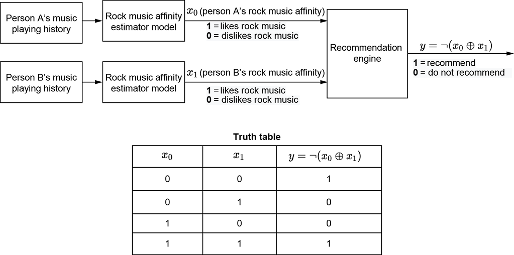
Figure 7.2 Example of logical NOT and XOR in a real-life problem. A social media system makes a friendship recommendation between persons A and B if and only if they both like or both dislike rock music. friendship = ¬ (rock-music-affinity-of-A ⊕ rock-music-affinity-of-B) where ¬ ⟹ logical NOT and ⊕ ⟹ logical XOR.
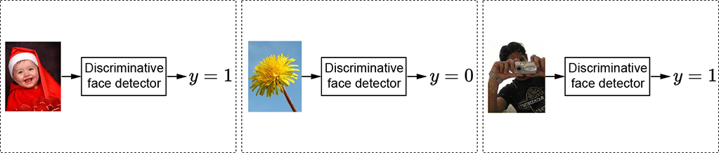
(a) Discriminative face detector classifier). The output is categorical (face or not face).
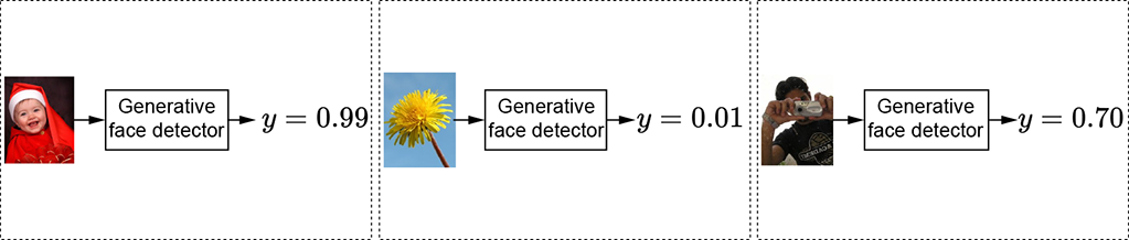
(b) Generative face detector. The output is continuous (the probability of an image containing a face).
Figure 7.3 The face detector takes an image as input and outputs a categorical or continuous variable.
7.2.2 Classifier functions in real-world problems
A classifier is a function whose output is categorical. Inputs can be either continuous or categorical. Thus, given an input, the function chooses one category (aka class) or another. For instance, a face detector can be a classifier. Its input is an image, and its output is a categorical (binary) variable that takes one of two possible values: 1 (face) or 0 (not face). This is shown in figure 7.3a. As we saw in section 2.3, any image can be represented by a vector ![]() . Accordingly, the classifier function for the face detectorcan be written as the function
. Accordingly, the classifier function for the face detectorcan be written as the function
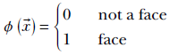
How to design the function ϕ(![]() ) is one of the primary topics of this chapter.
) is one of the primary topics of this chapter.
Geometrically, each scalar input variable forms a separate dimension in the input space. All possible combinations of these scalar input variables together form a multidimensional space called the input space (or feature space). Each specific combination of input values is a point (represented by the input vector ![]() ) in this space.
) in this space.
For instance, in an image, each pixel can be taken as a separate input scalar variable that can take any 3-byte pixel color value between RGB = ![]() ,
, ![]() ,
, ![]() (hex) (black) and RGB =
(hex) (black) and RGB = ![]() ,
, ![]() ,
, ![]() (hex) (white), with successive bytes (demarcated by an overline) representing red, green, and blue components of the pixel, respectively. The input has as many dimensions as the number of pixels in the image. For instance, a 224 × 224 image forms a 50, 176-dimensional input space. Each specific image is a single point in this space. The face-classifier function ϕ(
(hex) (white), with successive bytes (demarcated by an overline) representing red, green, and blue components of the pixel, respectively. The input has as many dimensions as the number of pixels in the image. For instance, a 224 × 224 image forms a 50, 176-dimensional input space. Each specific image is a single point in this space. The face-classifier function ϕ(![]() ) maps that point to either 0 (not face) or 1 (face).
) maps that point to either 0 (not face) or 1 (face).
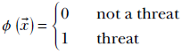
For a simpler instance, consider our familiar cat brain example from section 1.4. There are two input variables: x0, indicating hardness; and x1, indicating sharpness. The overall input space is two-dimensional, in which a specific input combination is denoted by the 2D vector ![]() . Our goal is to construct a machine that, given any input combination of hardness and sharpness, classifies it as either threatening or nonthreatening. This is equivalent to designing a function that maps arbitrary input vectors
. Our goal is to construct a machine that, given any input combination of hardness and sharpness, classifies it as either threatening or nonthreatening. This is equivalent to designing a function that maps arbitrary input vectors ![]() ∈ ℝ2 to 0 or 1:
∈ ℝ2 to 0 or 1:
Geometrical view of classifiers: Decision boundaries
Geometrically speaking, a classifier partitions the feature space into separate regions, each corresponding to a class. For instance, consider the simple cat-brain model from section 1.4. There are two input variables, hardness (x0) and sharpness (x1). Hence we have a two-dimensional input feature space that geometrically corresponds to a plane. Each combination of hardness and sharpness is represented by a specific vector ![]() = [x0, x1] corresponding to a point on the plane. Note that unlike the machines shown in figures 7.1a and 7.1b, here we are talking about a machine that takes as input a pair of continuous values hardness and sharpness)—that is, a point on the two-dimensional feature plane—and maps it to a discrete space corresponding to the threat versus not a threat categorical decision. This is illustrated in figure 7.4a.
= [x0, x1] corresponding to a point on the plane. Note that unlike the machines shown in figures 7.1a and 7.1b, here we are talking about a machine that takes as input a pair of continuous values hardness and sharpness)—that is, a point on the two-dimensional feature plane—and maps it to a discrete space corresponding to the threat versus not a threat categorical decision. This is illustrated in figure 7.4a.
The solid curve separates the threat and not-threat regions. Such curves that separate regions in input space belonging to different classes are known as decision boundaries. Estimating the decision boundary is effectively the same as building the classifier.
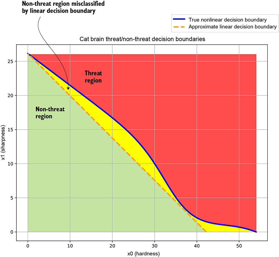
(a) Cat brain threat model decision boundary. The solid curve corresponds to the true decision boundary separating the threat and non-threat regions. The dashed line represents an approximate linear decision boundary: it classifies most points correctly but misclassifies points in the region between itself and the true decision boundary.
In practice, we get some sample points from each region through manual labeling.
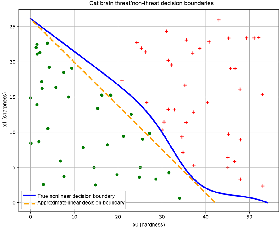
(b) Good training data. Sample points from each class roughly span the region of input space belonging to the class. This yields a good decision boundary (solid line).
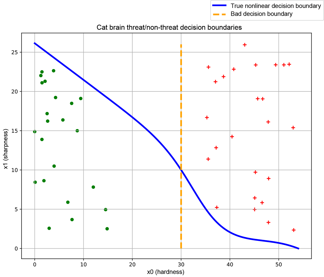
(c) Bad training data. Sample points from individual classes do not span the region of input space belonging to the class. This yields a bad decision boundary (dashed line).
Figure 7.4 Classifiers, decision boundaries, and training data. Data points from different classes are marked with different symbols (plus and dot).
The dashed line represents an approximate linear decision boundary that does the job crudely but misclassifies the points between the solid and dashed curves. (Linear decision boundaries are easier to represent with neural networks, but they are inadequate for complex problems.)
Let’s look briefly at the solid curve in figure 7.4a. At low hardness values, the sharpness threshold is high (if the object in front of the cat is not very hard, it must be very sharp to qualify as a threat). As hardness increases from x0 = 0 to x0 = 20, this threshold the sharpness required to qualify as a threat) drops more or less linearly. Beyond x0 = 20, the threshold drops at a much faster pace—if the object in front of the cat is sufficiently hard, it need not be very sharp to pose a threat. Beyond x0 = 52 or so, sharpness ceases to matter: sufficiently hard objects are threats even if they are not sharp. This is inherently a nonlinear situation.
To simplify neural network implementation, we might want to approximate the solid curve with a straight line—the dashed line is not too bad an approximation—but doing so entails errors. As shown in figure 7.4a, the region between the true and approximate curves will be wrongly classified.
Figure 7.4a is only a schematic. In reality, we do not know the exact regions in the input space that correspond to the classes of interest. We identify—via human labeling—some sample points on the input space, along with their correct class (the ground truth). Such a sampled set of <input point, correct output aka ground truth> pairs is called training data. An example training data set for the cat brain problem is shown in figure 7.4b (ground-truth training data points from different classes are marked with separate symbols: plus and dot, respectively). The decision boundary we create by training a neural network is optimized to classify the training data points (and nothing more) as nicely as possible. If the training data points’ distribution is a reasonable reflection of the true distribution—that is, the sample points from each class more or less span the entire region in the input space corresponding to that class—the decision boundary obtained by training on that data set will be good. But if, as illustrated in figure 7.4c, the training data does not reflect the true distribution of the classes in the input space, the decision boundary learned by training on that data maybe bad.
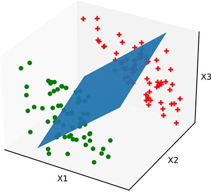
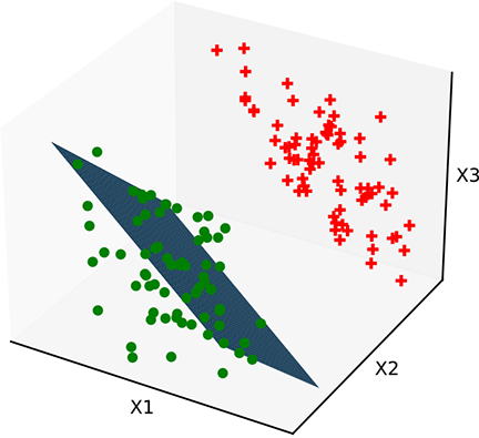
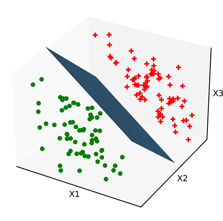
Unlike the cat brain example, most real-life input spaces have hundreds or even thousands of dimensions. The idea of a decision boundary as a hypersurface continues to hold in higher dimensions. For higher-dimensional input spaces, hyperplanes function as linear separators. In simpler problems with higher-dimensional input spaces, such linear separators suffice. In more complicated cases, we can have other curved hypersurfaces as nonlinear separators. We may not be able to visualize hyperspaces in our head, but we can form mental pictures with 3D analogs. Figure 7.5 shows some planar decision boundaries in 3D input space.
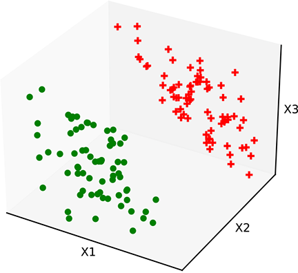
(a) Training data. Sample points from regions on the input space for each class
(b) Bad decision boundary. The plane has the wrong orientation. ![]() needs to be fixed.
needs to be fixed.
(c) Bad decision boundary. The plane has the correct orientation but the wrong position. b needs to be fixed.
(d) Optimal decision boundary. The plane has correct ![]() , b. Properly trained.
, b. Properly trained.
Figure 7.5 Classifiers with a linear decision boundary hyperplane). Such decision boundaries are created by perceptrons introduced in section 7.3.3). Data points from different classes are marked with different symbols plus and dot).
Figure 7.5a shows a 3D space of input vectors along with a set of training data points. The task is to classify them into two classes. In this simple situation, the training points can be partitioned with a hyperplanar decision boundary. Figures 7.5b and 7.5c show some planes that partition the training data poorly, and figure 7.5d shows an optimal planar separator. The only differences between these planes are the values of ![]() and b. This indicates that there are values of
and b. This indicates that there are values of ![]() and b that optimally partition the training data. These optimal values are determined by a process called training, which we discuss in detail in the nextchapter.
and b that optimally partition the training data. These optimal values are determined by a process called training, which we discuss in detail in the nextchapter.
Significance of sign: Mathematical expressions for decision boundaries
In a space with input vectors ![]() , the equation ϕ(
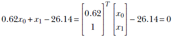
, the equation ϕ(![]() ) = 0 represents a surface. If the space is 2D, the surface becomes a curve. For instance, the straight dashed line in figure 7.4b can be viewed as a special case of ϕ(
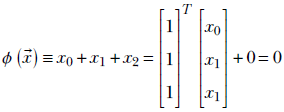
) = 0 represents a surface. If the space is 2D, the surface becomes a curve. For instance, the straight dashed line in figure 7.4b can be viewed as a special case of ϕ(![]() ) ≡
) ≡ ![]() T
T![]() + b = 0, which in this case becomes
+ b = 0, which in this case becomes
That is,

In 3D, we have surfaces like planes and spheres. In more than three dimensions, we have hyperplanes, hyperspheres, and so on. For instance, the plane in figure 7.6 corresponds to
Equation 7.1
That is,
In section 3.1.4, we saw that given any point ![]() in the space, the sign of ϕ(
in the space, the sign of ϕ(![]() ) tells us which side of the surface ϕ(
) tells us which side of the surface ϕ(![]() ) = 0 the point
) = 0 the point ![]() belongs to. Thus, if we estimate the surface corresponding to the decision boundary, given any point, we can determine the partition to which that point belongs. In other words, we can classify the point. Estimating the decision boundary is equivalent to building the classifier. For instance, the line in figure 7.4b corresponds to 0.62x0 + x1 − 26.14 = 0. The points with 0.62x0 + x1 − 26.14 < 0 are on one side and are indicated with dots. The points with 0.62x0 + x1 − 26.14 > 0 are on the other side and indicated with plus signs (+).
belongs to. Thus, if we estimate the surface corresponding to the decision boundary, given any point, we can determine the partition to which that point belongs. In other words, we can classify the point. Estimating the decision boundary is equivalent to building the classifier. For instance, the line in figure 7.4b corresponds to 0.62x0 + x1 − 26.14 = 0. The points with 0.62x0 + x1 − 26.14 < 0 are on one side and are indicated with dots. The points with 0.62x0 + x1 − 26.14 > 0 are on the other side and indicated with plus signs (+).
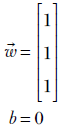
The idea extends to higher dimensions. Figure 7.6 shows the same idea in a 3D input space. The plane corresponds to the equation x0 + x1 + x2 = 0. The points with x0 + x1 + x2 < 0 are on one side (indicated by – in figure 7.6), and points with x0 + x1 + x2 > 0 are on the other side (indicated by + in figure 7.6).
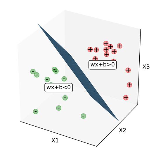
Figure 7.6 Significance of sign for ϕ(![]() ) ≡
) ≡ ![]() T
T![]() + b. Note that ϕ(
+ b. Note that ϕ(![]() ) = 0 implies that
) = 0 implies that ![]() lies on the plane, ϕ(
lies on the plane, ϕ(![]() ) negative implies one side of the plane, and ϕ(
) negative implies one side of the plane, and ϕ(![]() ) positive implies the other side of the plane.
) positive implies the other side of the plane.
7.2.3 General functions in real-world problems
There are problems where a categorical output variable will not do and a continuous output variable is called for: for instance, estimating the speed at which a self-driving vehicle should run. Using inputs like the speed limit for the road being traversed, speeds of neighboring vehicles, and so on, we need to estimate how fast the self-driving vehicle should go.
Another noteworthy situation where the output needs to be a continuous rather than a categorical variable is when we are modeling the probability of some event occurring. For instance, let’s again consider the face detector. Given an image as input, the face classification function emits 0 to indicate not a face and 1 to indicate face. Such functions are called discriminative. We could also have a function that outputs the probability of the image containing a face. Such functions are called generative, and an example is shown in figure 7.6.
7.3 The basic building block or neuron: The perceptron
In section 7.2, we saw that most real-world problems can be expressed as functions. This is good news, but the bad news is that these functions are usually unknown, and the functions underlying various problems are wildly different from each other. It may be possible to estimate them, but if we attack them individually without adopting a generic framework, there is little hope of developing a repeatable solution.
Neural networks provide an effective framework that can mechanically model an extremely wide variety of complicated functions. Furthermore, the target function need not be known in a closed form—sample input-output pairs are enough. They can represent (model) very complicated functions by connecting instances of a fairly simple building block, unsurprisingly called a neuron. In other words, the complete neural network can have huge expressive power even though a single neuron is very simple. Later, in sections 7.3.4, 7.4, 7.5, and so on, we discuss how neural networks model functions of increasing complexity. But first, in this section, we examine the building block: the neuron.
7.3.1 The Heaviside step function
The Heaviside step function, often referred to as simply the step function, is a function that takes the value 0 for negative arguments and the value 1 for positive arguments:
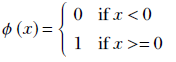
Equation 7.2
Equation 7.2 is equivalent to the following algorithm. Figure 7.7 shows the graph of this equation.
Algorithm 7.4 Heaviside step function as an algorithm
if x < 0 then
return 0
else
return 1
end if
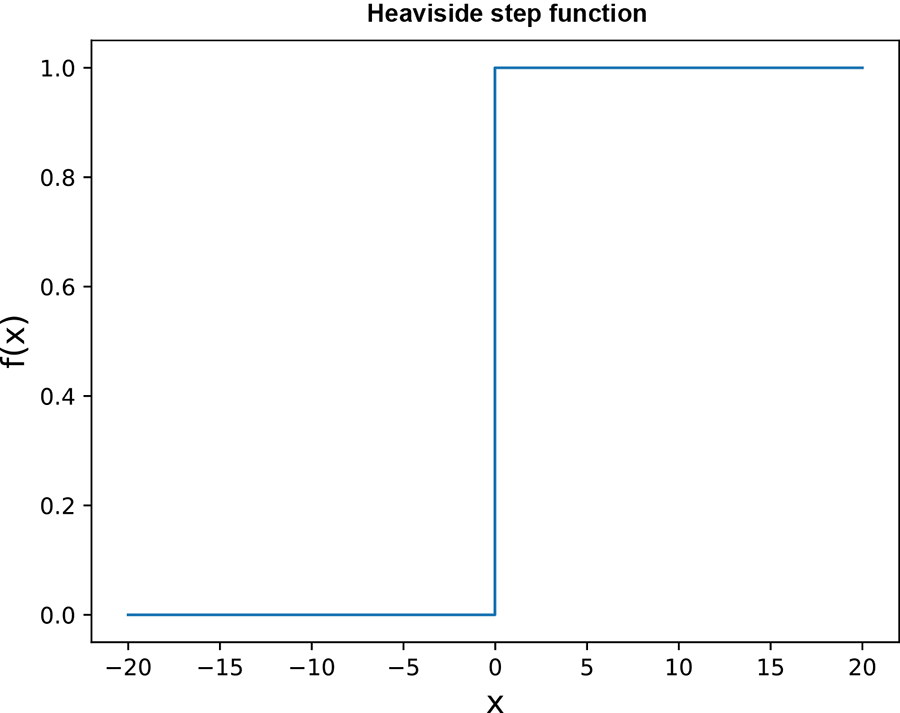
Figure 7.7 Heaviside step function graph
7.3.2 Hyperplanes
In section 2.8, we discussed hyperplanes. They are represented by equation 2.14. In figure 2.9, we saw the role that hyperplanes play in classifiers; we briefly revisit the idea here.
In section 2.1.1, we saw that d-element vectors are geometrical analogs of points in a d-dimensional space. Let ![]() denote the vectors (or, equivalently, points) in the space of input vectors. For a fixed vector
denote the vectors (or, equivalently, points) in the space of input vectors. For a fixed vector ![]() and fixed scalar b, the equation for a hyperplane in that space is
and fixed scalar b, the equation for a hyperplane in that space is
![]() T
T![]() + b = 0
+ b = 0
(meaning all points ![]() satisfying this equation lie on the plane). The vector
satisfying this equation lie on the plane). The vector ![]() is the normal to the plane. This becomes intuitively obvious when we observe that if we take any two points on the plane, say
is the normal to the plane. This becomes intuitively obvious when we observe that if we take any two points on the plane, say ![]() 0 and
0 and ![]() 1, then
1, then
![]() T
T![]() 0 + b = 0
0 + b = 0
![]() T
T![]() 1 + b = 0
1 + b = 0
Subtracting, we get
![]() T(
T(![]() 1 -
1 - ![]() 0) = 0
0) = 0
But (![]() 1 -
1 - ![]() 0) is the vector joining two arbitrary points on the plane. This means the line joining any pair of points on the plane is perpendicular to
0) is the vector joining two arbitrary points on the plane. This means the line joining any pair of points on the plane is perpendicular to ![]() (in section 2.5.2, we discussed dot products, and in section 2.6, we saw that if the dot product between two vectors is zero, the vectors are orthogonal—perpendicular to each other). Hence,
(in section 2.5.2, we discussed dot products, and in section 2.6, we saw that if the dot product between two vectors is zero, the vectors are orthogonal—perpendicular to each other). Hence, ![]() is orthogonal to all lines lying on the plane. In other words,
is orthogonal to all lines lying on the plane. In other words, ![]() is normal to the plane.
is normal to the plane.
The hyperplane ![]() T
T![]() + b = 0 partitions the space into two regions with distinct signs for the expression
+ b = 0 partitions the space into two regions with distinct signs for the expression ![]() T
T![]() + b. That is to say, the hyperplane can serve as a decision boundary, as shown in figure 7.6. Not just a hyperplane but any hypersurface can partition space in this fashion. This is true for any dimensionality of
+ b. That is to say, the hyperplane can serve as a decision boundary, as shown in figure 7.6. Not just a hyperplane but any hypersurface can partition space in this fashion. This is true for any dimensionality of ![]() :
:
-
If the expression
 T
T + b evaluates to zero, the point lies on the hyperplane T + b = 0.
 -
If the sign of the expression
T + b is negative, the point lies on one side of the hyperplane. -
If the sign of the expression
T + b is positive, the point lies on the other side of the hyperplane.
7.3.3 Perceptrons and classification
The perceptron combines the step function and a hyperplane into a single function. It represents the function
P(![]() ) ≡ ϕ(
) ≡ ϕ(![]() T
T![]() + b)
+ b)
Equation 7.3
where ϕ is the Heaviside step function from equation 7.2. Combining our insights from sections 7.3.1 and 7.3.2, we can see that the perceptron function maps all points on one side of the (![]() , b) plane to zero and all points on the other side of the same plane to 1. In other words, it performs as a linear classifier, with the (
, b) plane to zero and all points on the other side of the same plane to 1. In other words, it performs as a linear classifier, with the (![]() , b) plane as the decision boundary. Figure 7.8 graphs the perceptron function for a 2D input space (the graph itself is in 3D space: it maps points on one side of the decision boundary to the plane Z = 0 and points on the other side to the plane Z = 1).
, b) plane as the decision boundary. Figure 7.8 graphs the perceptron function for a 2D input space (the graph itself is in 3D space: it maps points on one side of the decision boundary to the plane Z = 0 and points on the other side to the plane Z = 1).
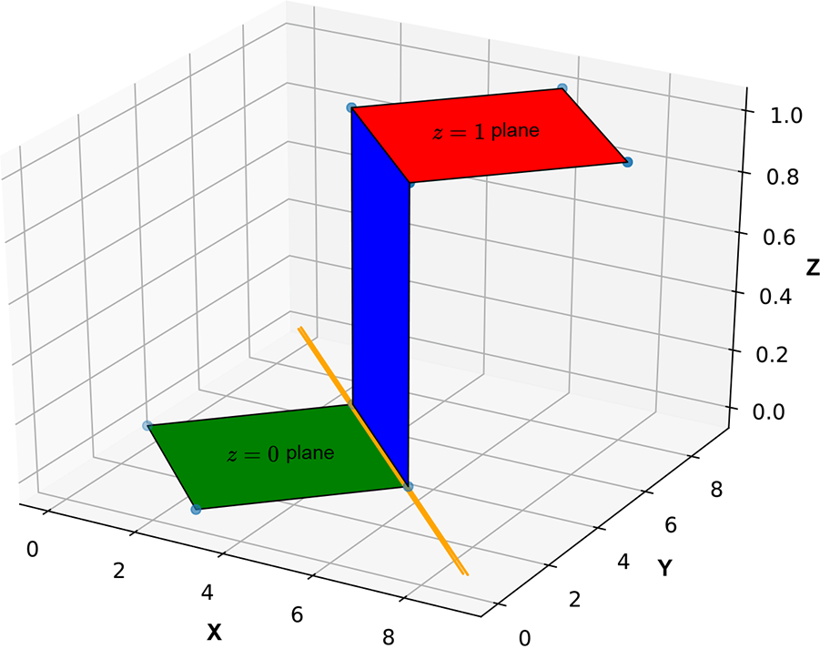
Figure 7.8 although the input space is 2D, the perceptron graph is 3D. The decision boundary is indicated by the long diagonal straight line. It maps points on one side of the decision boundary to the Z = 0 plane and the points on the other side to the Z = 1 plane.
Of course, in real life, we do not know the exact regions corresponding to classes. Rather, we have sampled input points with their manually labeled classes as training data. The decision surface must be constructed based on this training data only. In figure 7.4, we saw an example decision boundary in 2D along with some good and bad training data sets. To get a mental picture of sampled training data sets in higher dimensions, look at figure 7.5a again. In this simple situation, a single hyperplanar decision boundary is sufficient to partition the training points. This means a single perceptron-based neural network will suffice as a classifier. Figures 7.5b and 7.5c depict some planes (perceptrons with specific (![]() , b) values) that poorly partition the training data. Figure 7.5d shows an optimal perceptron (planar separator). This tells us that there are good values of
, b) values) that poorly partition the training data. Figure 7.5d shows an optimal perceptron (planar separator). This tells us that there are good values of ![]() and b that optimally partition the training data, as well as bad values. As mentioned earlier, good values are determined through training, which we cover in chapter 8.
and b that optimally partition the training data, as well as bad values. As mentioned earlier, good values are determined through training, which we cover in chapter 8.
The perceptron effectively partitions with a planar decision surface. This works only in simple problems. For an instance of a situation where a planar decision surface will not work, see figure 7.9. It depicts a problem where one class maps to the set of points sandwiched between two planes and the other class to the rest of the points in the input space. It is impossible to achieve the required partitioning with a single plane, so such a decision boundary cannot be modeled with a single perceptron. Later we will see how to model such complex decision boundaries with multiple perceptrons.
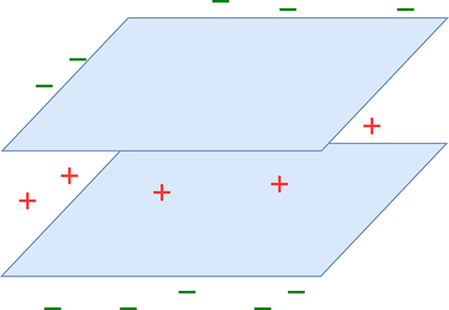
Figure 7.9 Multiplane decision boundary. One class corresponds to the points in the region sandwiched between the planes (marked +). The remaining points correspond to the other class marked –). This decision boundary cannot be represented with a single plane.
NOTE Fully functional code for perceptrons, executable via Jupyter Notebook, can be found at http://mng.bz/9Ne7.
The following listing shows the PyTorch code for a perceptron.
Listing 7.1 Perceptron
def fully_connected_layer(X, w,  b):                         ①

    X = torch.cat((X, torch.ones(
             [X.shape[0], 1], dtype=torch.float32)), dim=1)  ②

    W = torch.cat((W, b.unsqueeze(dim=1)), dim=1)            ③

    y = torch.matmul(W, X.transpose(0, 1))                   ④

    y = torch.heaviside(y, torch.tensor(1.0))                ⑤

    return y.transpose(0, 1)

def Perceptron(X, W, b):                                     ⑥
    return fully_connected_layer(X, W, b)
① X : n × d tensor; each row is an input vector of size d. w : m × d tensor.
② Adds a column of 1s. X ↦ n × (d+1) tensor.
③ Combines weights and biases
④ Matrix multiplication of X and W
⑤ Applies the Heaviside step function
⑥ A single perceptron
7.3.4 Modeling common logic gates with perceptrons
Neural networks provide a structured way of modeling complex functions by connecting—via weighted edges—repeated instances of a simple building block called the perceptron. In this section, we explore the idea of function modeling via perceptrons. We start with modeling extremely simple logical functions (AND, OR, NOT, voting) that can be represented with single perceptrons. Then we look at the XOR function, one of the simplest functions that cannot be represented with a single perceptron; we see that it can be modeled with multiple perceptrons. Next we discuss Cybenko’s theorem, which states that most functions of interest can be modeled with as much accuracy as we want via perceptrons, with a single hidden layer between inputs and outputs. Unfortunately, this is less practical than it sounds: the catch is that although any function can be modeled to any accuracy, there is no limit on how many perceptrons are required to do the modeling. The more complicated the target function is, the more perceptrons are required. In practice, we often use many layers instead of one.
A perceptron for logical AND
Figure 7.18 depicts this perceptron. It takes two inputs, x0 and x1, which are weighted with w0 = 1 and w1 = 1, respectively; the bias is −1.5 actually, a wide range of bias values will do). Overall, the perceptron implements the function ϕ(x0 + x1−1.5). This function emits 1 when x0 + x1 − 1.5 ≥ 0: that is, x0 + x1 ≥ 1.5. Since the variables are binary (meaning they can only take the value 0 or 1), this can happen only when both inputs are 1. If either is zero, their sum is less than 1.5, and y is 0.
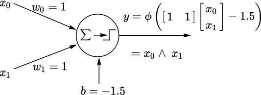
(a) Perceptron for a logical AND function: y = x0 ∨ x1
(b) Perceptron for a logical OR function: y = x0 ∧ x1
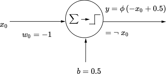
(c) Perceptron for a logical NOT function: y = ¬x0
Figure 7.10 functions are binary, meaning they can be either 0 or 1.
The situation is depicted geometrically in figure 7.11a. The thick diagonal line corresponds to x0 + x1 ≥ 1.5. It partitions the plane into unshaded and shaded All points on the unshaded half-plane have an output value y = 0, and all points on the shaded half-plane have the output value y = 1. There are only four possible input points: (x0 = 1, x1 = 1), (x0 = 1, x1 = 1), (x0 = 1, x1 = 1), (x0=1, x1 = 1). The point (x0=1, x1 = 1) falls on the shaded side and the others on the unshaded side—which is exactly the logical AND function.
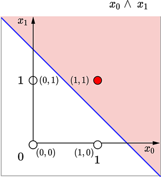
(a) Logical AND decision boundary: x0 + x1 = 1.5
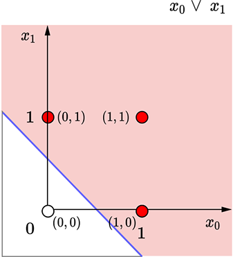
(b) Logical OR decision boundary: x0 + x1 = 0.5
(c) Logical NOT decision boundary: x0 = 0.5
Figure 7.11 Geometrical views for the perceptrons in figure 7.10. Each dot represents an input point(a [x0 x1] vector). The shaded dots map to an output value of 1, and the unshaded dots map to an output value of 0. The thick line indicates the decision boundary.
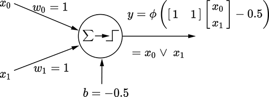
A perceptron for logical OR
Figure 7.10b depicts this perceptron. It takes two inputs, x0 and x1, which are weighted with w0 = 1 and w1 = 1, respectively; the bias is −0.5. Overall, the perceptron implements the function ϕ(x0 + x1−0.5). This function emits 1 when x0 + x1 − 0.5 ≥ 0: that is, x0 + x1 ≥ 0.5. Since the variables are binary (0 or 1), this can happen when either or both inputs are 1. If and only if both of them are zero, their sum is zero (less than 0.5), and y is 0.
The situation is shown geometrically in figure 7.11b. The thick line corresponds to x0 + x1 ≥ 0.5, partitioning the input plane into an unshaded half-plane (all points on this half-plane have output y = 0) and a shaded half-plane output y = 1). Of the four possible input points, (0,0) falls on the unshaded side (y = 1) and the remaining three on the shaded side (y = 1)—which is exactly the logical OR function.
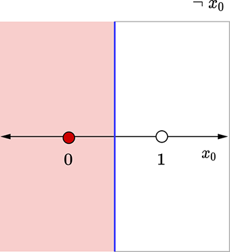
A perceptron for logical NOT
This perceptron is shown in figures 7.10c and 7.11c, which should be self-explanatory by now.
NOTE Fully functional code for modeling various logical gates using perceptrons, executable via Jupyter Notebook, can be found at http://mng.bz/jBRr.
Listing 7.2 Modeling logical gates using perceptrons
# Logical AND
X = torch.tensor([[0., 0.],                               ①
                 [0., 1.],
                 [1., 0.],
                 [1., 1.]], dtype=torch.float32)
W = torch.tensor([[1.0, 1.0]], dtype=torch.float32)       ②
b = torch.tensor([-1.5])                                  ③
Y = Perceptron(X=X, W=W, b=b, activation=torch.heaviside) ④

# Logical OR
X = torch.tensor([[0., 0.],
                 [0., 1.],
                 [1., 0.],
                 [1., 1.]], dtype=torch.float32)
W = torch.tensor([[1.0, 1.0]], dtype=torch.float32)
b = torch.tensor([-1.5])
Y = Perceptron(X=X, W=W, b=b, activation=torch.heaviside)

# Logical NOT
X = torch.tensor([[0],
                 [1.]
                 ], dtype=torch.float32)
W = torch.tensor([[-1.0]], dtype=torch.float32)
b = torch.tensor([0.5])
Y = Perceptron(X=X, W=W, b=b, activation=torch.heaviside)
① Input data points
② Instantiates the weights
③ Instantiates the bias
④ Output
7.4 Toward more expressive power: Multilayer perceptrons (MLPs)
There is a remarkably simple logical function that, somewhat surprisingly, cannot be modeled with a single perceptron: XOR. We discuss it now.
(a) Geometric view of the logical XOR perceptron. The decision boundary has two lines, so using a single perceptron is impossible.
(b) MLP for the logical XOR function. Note that weights and biases have superscripts in parentheses indicating the layer index. This is a two-layered network. Layer 0 is hidden.
Figure 7.12 Logical XOR: Geometric and perceptron view
7.4.1 MLP for logical XOR
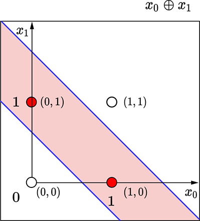
Figure 7.12a shows the four possible input points on the plane and how the plane needs to be partitioned to model the XOR function. The points (0,0), (1,1) (unshaded) both map to output 0 and should be on the same side of the decision boundary, while the points (0,1), (1,0) shaded) map to output value 1 and should be on the other side of the decision boundary.
It is easy to see that it is impossible to draw a single straight line in this plane such that the shaded points are on one side and the unshaded points are on the other. Remember, a perceptron essentially introduces a linear decision boundary. Hence it is impossible to have a single perceptron modeling this function.
However, it is possible to model the logical XOR function via multiple perceptrons. One such model is shown in figure 7.12b.
7.5 Layered networks of perceptrons: MLPs or neural networks
The XOR example tells us that we cannot do much with single perceptrons. We must connect more than one perceptron into a network to solve practical problems. This is a neural network. How do we organize such a network of connected perceptrons?
7.5.1 Layering
Layering is the most popular way to organize perceptrons into a neural network. Figure 7.12b is our first example of an MLP—most of the remainder of the book talks about MLPs.
Note how the perceptrons in the XOR network (figure 7.12b) are organized:
-
The layers are numbered with increasing integers from input to output.
-
The output of a perceptron in layer i is only fed as input to perceptrons in layer i + 1. No other connections are allowed. This keeps the network manageable andfacilitates updating the weights during training via a technique called backpropagation, which we discuss in the next chapter.
-
Outputs of all layers but the last are invisible (do not directly contribute tothe output). Such layers are called hidden layers. In figure 7.12b, layer 0 ishidden.
-
Each weight and bias element belongs to one and only one layer. Throughout this book, we indicate the layer index for a weight or bias element as a superscript within parentheses.
-
MLPs with two or more hidden layers can be called deep neural networks. This is the origin of the word deep in deep learning.
7.5.2 Modeling logical functions with MLPs
Any logical function can be expressed as a truth table. Hence, if we can prove that all truth tables can be implemented via MLPs, we are done. This is the approach we take here.
NOTE In the following discussion, no symbol (à la multiplication) between two variables indicates logical AND, and a + symbol indicates logical OR.
Table 7.1 Truth table for the logical function y = x̄0x1 ¸ x0x̄1
|
x0 |
x1 |
y |
|---|---|---|
|
0 |
0 |
0 |
|
0 |
1 |
1 |
|
1 |
0 |
1 |
|
1 |
1 |
0 |
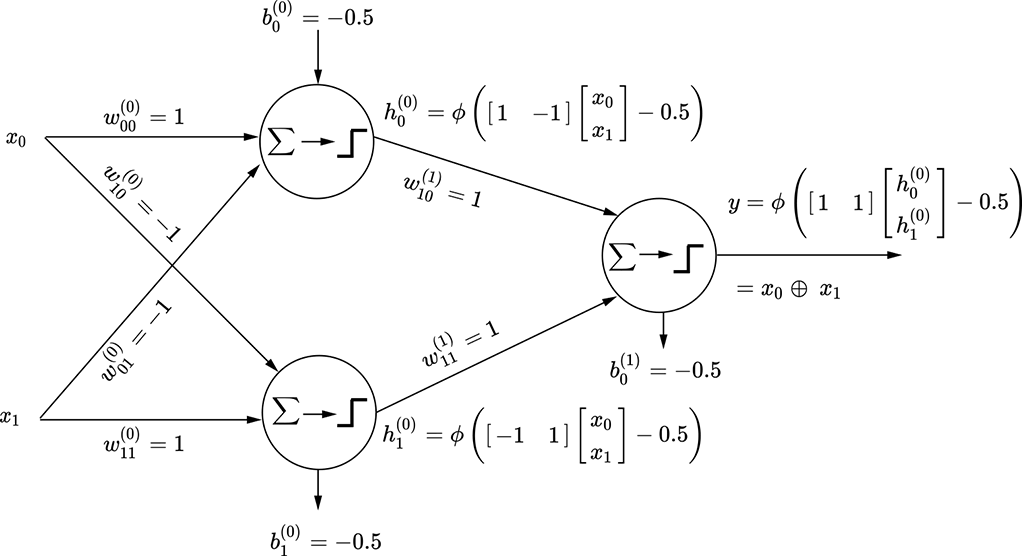
Let’s start with a simple two-variable logical functions y = x̄0x1 + x0x̄1. Table 7.1 shows the corresponding truth table. To create the equivalent MLP, we must pick the rows corresponding to y = 1. Each row can be expressed as an AND of the input variables or their complements. For instance, the row x0 = 0 and x1 = 1, y = 1 corresponds to x̄0x1—the first term of the function we are trying to implement—and can be implemented by the perceptron shown in figure 7.13a. The row x0 = 1 and x1 = 0, y = 1 corresponds to x0x̄1—the second term of the function we are trying to implement—and can be implemented by the perceptron shown in figure 7.13b. We have implemented the individual terms of the function; all that remains is to OR them together into a final MLP, as shown in figure 7.13c. This logical function is our old friend, logical XOR, and the overall function in figure 7.13 is the same as figure 7.12. In this fashion, arbitrary logical expressions in any number of variables can be modeled using MLPs.
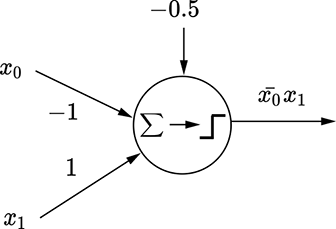
(a) Perceptron for x̄0x1

(b) Perceptron for x0x̄1
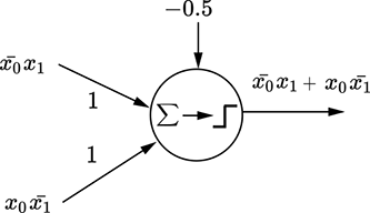
(c) MLP for x̄0x1 + x0x̄1
Figure 7.13 MLP for the logical function corresponding to table 7.1
Listing 7.3 Multilayered perceptron (MLP)
def MLP(X, W0, W1, b0, b1): ①
    y0 = fully_connected_layer(X=X, W=W0, b=b0)
    return fully_connected_layer(X=y0, W=W1, b=b1)
① MLP
7.5.3 Cybenko’s universal approximation theorem
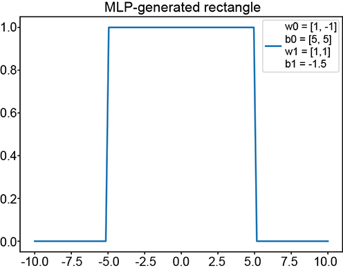
Any function y = f(x) that is continuous in an interval x ∈ (a, b) can be approximated with a set of towers (vertical rectangles) in that interval. This is a direct consequence of the mean value for integrals theorem in calculus. The idea is depicted in figure 7.14, where a complicated function (depicted by the curve) is approximated by a sequence of towers of various heights. The thinner the towers, the greater the number of towers, and the more accurate the approximation.
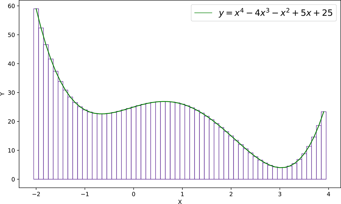
Figure 7.14 Approximating a complicated function with towers
In section 7.5.3.1, we show that any tower (with arbitrary height and location) can be constructed with MLPs. By summing these MLPs for individual towers, we can approximate the entire function. This is Cybenko’s theorem in a nutshell.
NOTE Although Cybenko’s theorem guarantees that any continuous function can be modeled using an MLP with a single hidden layer, the number of perceptrons in that MLP can become arbitrarily impracticably large. This is why, in real life, we rarely try to approximate complicated functions with a single hidden layer. We see later that additional layers help us cut down the number of perceptrons required.
In particular, any decision boundary can be modeled in this fashion. Of course, the number of perceptrons needed may become impossibly large for many problems, making such a model practically unattainable.
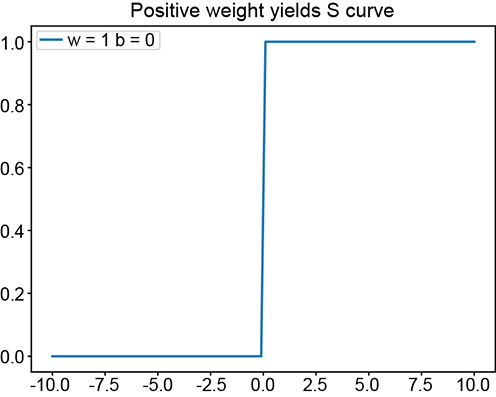
(a) ϕ(x): positive w yields a regular step
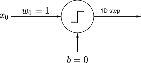
(b) Perceptron for a regular step
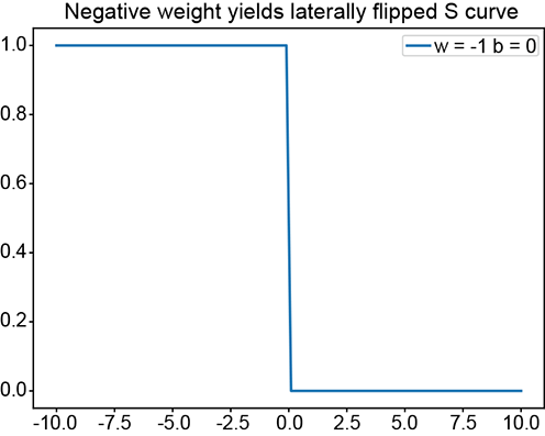
(c) ϕ(−x): negative w yields a laterally flipped step
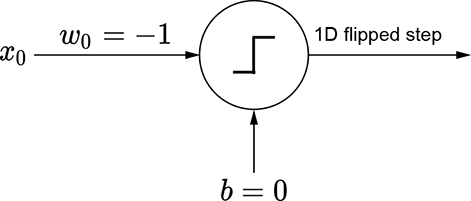
(d) Perceptron for a laterally flipped step
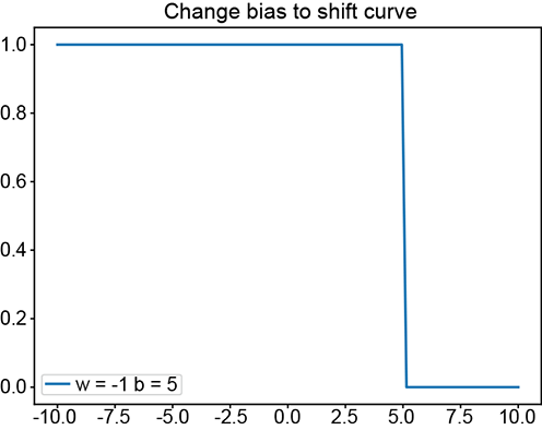
(e) ϕ(−x+5): changing the bias shifts the step left or right
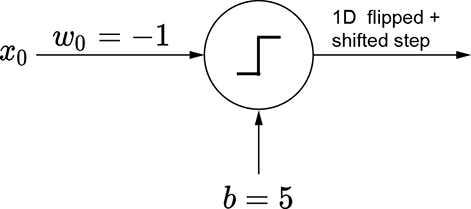
(f) Perceptron for a laterally shifted step
(g) (ϕ(x+5)+ϕ(−x+5)−1.5): ANDing a left-shifted step with a flipped, right-shifted step yields a tower
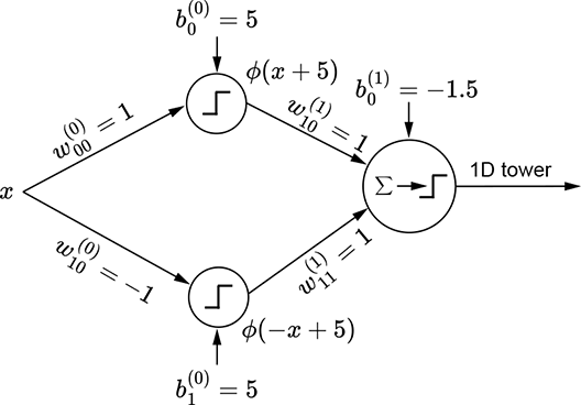
(h) MLP for a 1D tower
Figure 7.15 Generating a 1D tower with perceptrons.
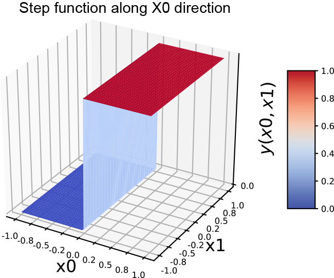
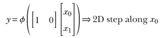
(a) 2D step function along the x0 (x) direction
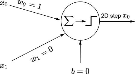
(b) Perceptron for a 2D step function along the x0 (x) direction
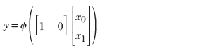
(c) Equation for a 2D step function along the x0 (x) direction
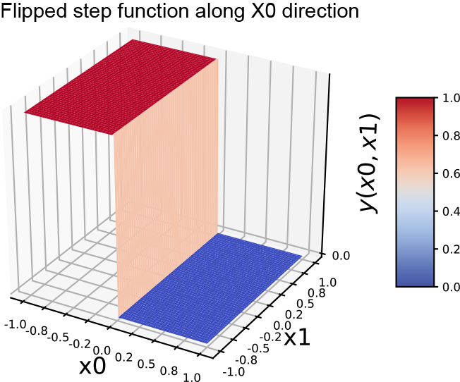
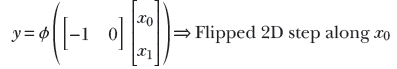
(d) Flipped 2D step along the x0 (x) direction
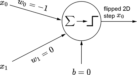
(e) Perceptron for a flipped 2D step along the x0 (x) direction
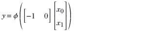
(f) Equation for a flipped 2D step along the x0 (x) direction
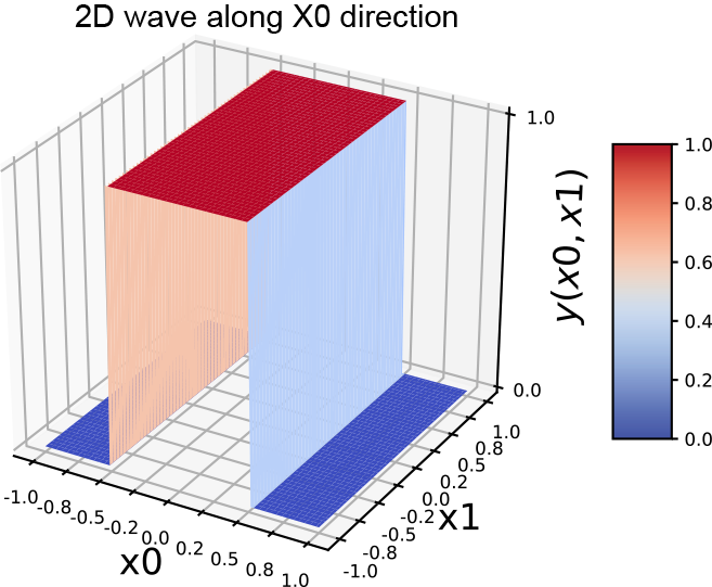
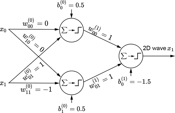
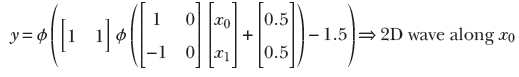
(g) 2D wave along the x0 x) direction
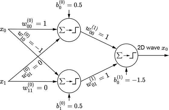
(h) MLP for a 2D wave along the x0 (x) direction
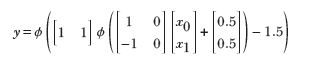
(i) Equation for a 2D wave along the x0 (x) direction
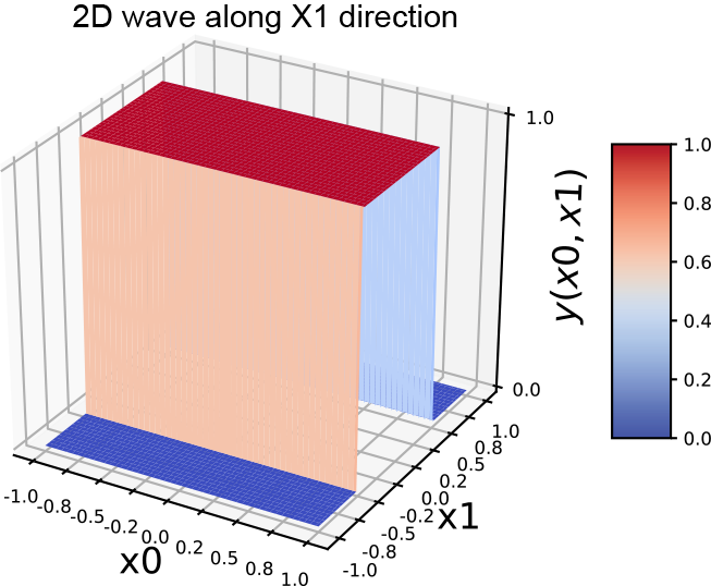
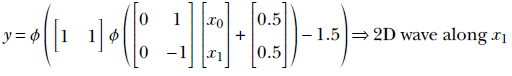
(j) 2D wave along the x1 y) direction
(k) MLP for a 2D wave along the x1 (y) direction
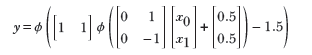
Figure 7.16 Generating 2D steps and waves with perceptrons.
Generating towers with MLPs
The basic idea is depicted in figure 7.15. We can obviously generate a regular step with a perceptron implementing y = ϕ(x). The corresponding graph is shown in figure 7.15a. By imparting a bias of 5, we can shift this step leftwards. The corresponding function is y = ϕ(x+5). Furthermore, using negative weight laterally flips the step. The corresponding function is y = ϕ(−x), whose graph is shown in figure 7.15c. By imparting a bias of 5, we can shift the flipped step rightwards. Figure 7.15e shows a flipped and right-shifted step corresponding to the function y = ϕ(−x+5), whose perceptron is shown in figure 7.15f. Logically ANDing a left-shifted step with a flipped and right-shifted step yields a tower in 1D. This corresponds to the function y = ϕ(ϕ(x+5)+ϕ(−x+5)−1.5), whose graph is shown in figure 7.15g.
The same idea also works for higher-dimensional inputs. We can generate a step in two variables (a 2D step) aligned to the x0 direction using equation 7.4. This equation’s graph is shown in figure 7.16a, and the perceptron implementing the equation is shown in figure 7.16b. The flipped version of the same step can be generated via equation 7.5. This equation’s graph is shown in figure 7.16d, and the perceptron implementation is shown in figure 7.16e.
In the 1D case, we combine a regular step with its flipped and shifted version to generate a tower. The process is slightly more complicated in 2D. Here, combining a step along a specific coordinate axis with its flipped and shifted version generates a wave function along that axis. Thus, we have separate waves in each dimension. The wave along the x0 axis corresponds to equation 7.6; its graph is shown in figure 7.16g. It is implemented by the MLP in figure 7.16h. Similarly, a 2D wave along the x1 axis can be generated via equation 7.7 and is graphed in figure 7.16j. The corresponding MLP is shown in figure 7.16k.
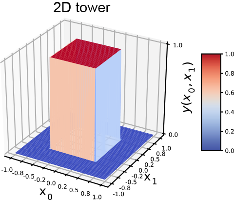
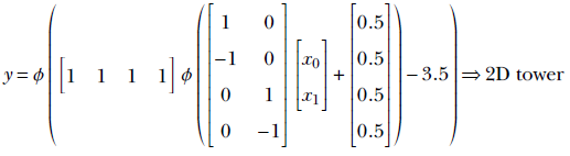
To create a tower, we have to AND a pair of waves along the two separate dimensions. The final tower function is shown in equation 7.8; the corresponding tower graph is shown in figure 7.17a; the MLP is shown in figure 7.17b. Any continuous 2D surface can be approximated to arbitrary levels of accuracy by combining such 2D towers:
(a) 2D tower
(b) MLP for a 2D tower (equation 7.8)
Figure 7.17 Generating a 2D tower with perceptrons
Equation 7.4
Equation 7.5
Equation 7.6
Equation 7.7
Equation 7.8
NOTE Fully functional code for approximating surfaces using perceptrons, executable via Jupyter Notebook, can be found at http://mng.bz/WrKa.
Listing 7.4 Perceptrons and MLPs in 1D
x = torch.linspace(start=-10, end=10, steps=100) ①

# 1D S curves - positive weight                  ②
w = torch.tensor([1.0], dtype=torch.float32)
b = torch.tensor([0.0])
y = Perceptron(X=x.unsqueeze(dim=1), W=w.unsqueeze(dim=1), b=b)

# 1D S curves - negative weight + shift\quad     ③
w = torch.tensor([-1.0], dtype=torch.float32)
b = torch.tensor([5.0])
y = Perceptron(X=x.unsqueeze(dim=1), W=w.unsqueeze(dim=1), b=b)

# 1D towers (Cybenko) - various W0\quad          ④
W0 = torch.tensor([[1.0], [-1.0]], dtype=torch.float32)
b0 = torch.tensor([5.0, 5.0])
W1 = torch.tensor([[1.0, 1.0]], dtype=torch.float32)
b1 = torch.tensor([0.0])
y = MLP(X=x.unsqueeze(dim=1), W0=W0, W1=W1, b0=b0, b1=b1)
① 100D array
② See figures 7.15a and 7.15b.
③ See figures 7.15e and 7.15f.
④ See figures 7.15g and 7.15h.
Listing 7.5 Perceptrons and MLPs in 2D
X = torch.linspace(start=-1, end=1, steps=100)      ①
Y = torch.linspace(start=-1, end=1, steps=100)      ①

gridX, gridY = torch.meshgrid(X, Y)                 ②
X = torch.tensor([(y, x) for y, x in
         zip(gridY.reshape(-1), gridX.reshape(-1))) ③

# 2D Step function in X-direction                   ④
W = torch.tensor([[1.0, 0.0]], dtype=torch.float32)
b = torch.tensor([0.0], dtype=torch.float32)
Z = Perceptron(X=X, W=W, b=b)

# 2D Flipped Step function along X-direction        ⑤
W = torch.tensor([[-1.0, 0.0]], dtype=torch.float32)
b = torch.tensor([0.0], dtype=torch.float32)
Z = Perceptron(X=X, W=W, b=b)

# 2D wave along X-direction                         ⑥
W0 = torch.tensor([[1.0, 0.0],
                   [-1.0, 0.0]], dtype=torch.float32)
b0 = torch.tensor([0.5, 0.5], dtype=torch.float32)
W1 = torch.tensor([[1.0, 1.0]], dtype=torch.float32)
b1 = torch.tensor([-1.0])
Z = MLP(X=X, W0=W0, W1=W1, b0=b0, b1=b1)

# 2D wave along Y-direction                          ⑦
W0 = torch.tensor([[0.0, 1.0],
                   [0.0, -1.0]], dtype=torch.float32)
b0 = torch.tensor([0.5, 0.5], dtype=torch.float32)
W1 = torch.tensor([[1.0, 1.0]], dtype=torch.float32)
b1 = torch.tensor([-1.0])
Z = MLP(X=X, W0=W0, W1=W1, b0=b0, b1=b1)

# 2D Tower                                           ⑧
W0 = torch.tensor([[1.0, 0.0],
                   [-1.0, 0.0],
                   [0.0, 1.0],
                   [0.0, -1.0]], dtype=torch.float32)
b0 = torch.tensor([0.5, 0.5, 0.5, 0.5], dtype=torch.float32)
W1 = torch.tensor([[1.0, 1.0, 1.0, 1.0]], dtype=torch.float32)
b1 = torch.tensor([-3.5])
Z = MLP(X=X, W0=W0, W1=W1, b0=b0, b1=b1)
① 100D array
② 100 × 100 matrix
③ 10,000 × 1 matrix
④ See equation 7.4 and figures 7.16a and 7.16b
⑤ See equation 7.5 and figures 7.16d and 7.16e
⑥ See equation 7.6 and figures 7.16g and 7.16h
⑦ See equation 7.7 and figures 7.16j and 7.16k
⑧ See equation 7.8 and figures 7.17a and 7.17b
7.5.4 MLPs for polygonal decision boundaries
We have seen that classifiers form an important use case for neural networks. In section 7.2.2.1, we also saw that classifiers essentially model decision boundaries in high-dimensional feature spaces. In this section, we model a simple class bounded with a fixed polygon to understand the process.
Figure 7.18a shows a feature space with the class to be identified corresponding to a rectangular region (shaded) bounded by the four straight lines:
x0 = –5 x0 = 5
x1 = –2 x1 = 2
Each of these lines partitions the feature space into two half-planes, indicated by minus and plus signs in figure 7.18a. The region containing the feature points for the class of interest is indicated by all + signs.
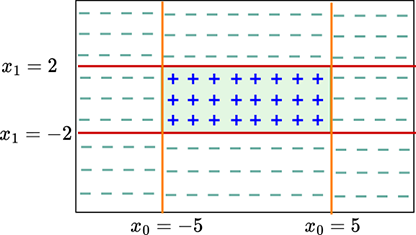
(a) Example feature space with decision boundaries enclosing the class of interest (shaded)
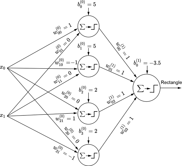
(b) MLP that fires only on points in the shaded region
Figure 7.18 Modeling a rectangular decision region with MLPs
The shaded region corresponding to the class of interest is the region where x0 ≥ − 5 AND x0 ≤ 5 AND x1 ≥ − 2 AND x1 ≤ 2. Now consider the perceptron ϕ(x0+5). It fires (outputs 1) on the region x0 ≥ − 5. Similarly, the perceptrons ϕ(−x0+5), ϕ(x1+2), and ϕ(−x1+2) fire on the regions x0 ≤ 5, x1 ≥ − 2, and x1 ≤ 2, respectively. Hence, by logically ANDing the outputs of these perceptrons, we get an MLP that fires only on the shaded region of interest. Figure 7.53 shows this MLP. It implements the following function:
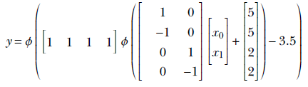
All shapes on a plane can be approximated by polygons. Hence, given sufficient perceptrons, any shape on a plane can be depicted to an arbitrary level of accuracy.
Summary
In this chapter, we outlined how a large variety of real-world problems can be modeled as function evaluation:
-
Any intelligent task can be modeled by a function. Of particular interest are classification tasks where, given an input, we estimate from a predetermined list of possible classes the class to which the input belongs. For instance, a binary classifier can group input images into two classes: those that contain a human face and those that do not. Classification tasks can be approximated by functions with categorical outputs.
-
Neural networks provide a structured way to approximate arbitrary functions (including classifier functions). This is how they mimic intelligence.
-
Neural networks are created by combining a basic building block called a perceptron. A perceptron is a simple function that returns a step function applied to the weighted sum of its inputs (plus a bias). A perceptron is effectively a linear classifier that divides space into two half-spaces with a hyperplane. The weights and bias of the perceptron correspond to the orientation and position of the hyperplane—they can be adjusted to separate the regions corresponding to individual classes as much as possible.
-
A single perceptron can approximate only relatively simple functions, such as a classifier whose feature points are separable by a hyperplane. Perceptrons cannot approximate more complex functions, like classifiers whose input regions are to be separated with curved surfaces. Multilayer perceptrons (MLPs) are combinations of perceptrons where the outputs of one set (layer) of perceptrons are fed as input to the next set (layer). A neural network is essentially an MLP and can approximate such arbitrarily complex functions.
-
Simple logical functions like AND, OR, and NOT can be emulated with a single perceptron. A logical XOR cannot be. For XORs and other complicated logical functions, we need MLPs. There is a mechanical way to construct an MLP for any logical function. A logical function can always be represented by a truth table. Each row of the truth table can be viewed as a logical AND function of the inputs, and the final output is a logical OR of the inputs. Since ANDs and ORs can be emulated with perceptrons, any truth table can be emulated as a combination of perceptrons (an MLP).
-
The ability of an MLP to represent arbitrary functions is known as its expressive power. The larger the number of perceptrons and/or connections, the greater the expressive power of a neural network.
-
Cybenko’s theorem proves that a neural network is a universal approximator (meaning it can approximate any function). The basic idea is that any function can be approximated to an arbitrary degree of accuracy as a sum of rectangles (towers). The theorem demonstrates that a tower can be constructed in any dimensional space using MLPs.
-
Neural networks can approximate any shape on a plane to arbitrary accuracy. This is because all shapes can be approximated by rectangles, and we can demonstrably approximate a rectangle on a plane with MLPs.
-
In real-life problems, the regions corresponding to classes are unknown, but we manually label sample input points with desired outputs (ground truth) to create supervised training data. We tune the weights and biases to approximate the training data as closely as possible. This process of tuning is known as training. If the training data set is not a good representative of the real dataset, the neural network will be inaccurate even after training.