8 Training neural networks: Forward propagation and backpropagation
This chapter covers
- Sigmoid functions as differential surrogates for Heaviside step functions
- Layering in neural networks: expressing linear layers as matrix-vector multiplication
- Regression loss, forward and backward propagation, and their math
So far, we have seen that neural networks make complicated real-life decisions by modeling the decision-making process with mathematical functions. These functions can become arbitrarily involved, but fortunately, we have a simple building block called a perceptron that can be repeated systematically to model any arbitrary function. We need not even explicitly know the function being modeled in closed form. All we need is a reasonably sized set of sample inputs and corresponding correct outputs. This collection of input and output pairs is known as training data. Armed with this training data, we can train a multilayer perceptron (MLP, aka neural network) to emit reasonably correct outputs on inputs it has never seen before.
Such neural networks, where we need to know the output for each input in the training data set, are known as supervised neural networks. The correct output for the training inputs is typically generated via a manual process called labeling. Labeling is expensive and time-consuming. Much research is going on toward unsupervised, semi-supervised, and self-supervised networks, eliminating or minimizing the labeling process. But as of now, the accuracy of unsupervised and self-supervised networks in general does not match that of supervised networks. In this chapter, we focus on supervised neural networks. In chapter 14, we will study unsupervised networks.
What is this process of “training” a neural network? It essentially estimates the parameter values that would make the network emit output values as close as possible to the known correct outputs on the training inputs. In this chapter, we discuss how this is done. But before that, we have to learn a few other things.
NOTE The complete PyTorch code for this chapter is available at http://mng.bz/YAXa in the form of fully functional and executable Jupyter notebooks.
8.1 Differentiable step-like functions
In equation 7.3, we expressed the perceptron as a combination of a Heaviside step function ϕ and an affine transformation ![]() T
T![]() + b. This is the perceptron we used throughout chapter 7 and with which we were able to express (model) pretty much all functions of interest.
+ b. This is the perceptron we used throughout chapter 7 and with which we were able to express (model) pretty much all functions of interest.
Despite its expressive power, the Heaviside step function has a drawback: it has a discontinuity at x = 0 and is not differentiable. Why is differentiability important? As we shall see in chapter 8 (and got a glimpse of in section 3.3), optimal training of a neural network requires evaluation of the gradient vector of a loss function with respect to weights. Since the gradient is nothing but a vector of partial derivatives, differentiability is needed for training.
In this section, we discuss a few functions that are differentiable and yet can mimic the Heaviside step function. The most significant among them is the sigmoid function.
8.1.1 Sigmoid function
The sigmoid function is named after its characteristic S-shaped curve figure 8.1). The corresponding equation is
![]()
Equation 8.1
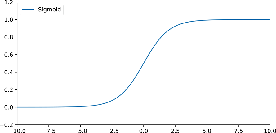
Figure 8.1 Graph of a 1D sigmoid function
Parameterized sigmoid function
We can parametrize equation 1.5 as
![]()
Equation 8.2
This allows us to
-
Adjust the steepness of the linear portion of the S curve by changing w
-
Adjust the position of the curve by changing b
Figure 8.2 shows how the parametrized sigmoid curve changes with different values for the parameters w and b. In particular, note that for large values of w, the parameterized sigmoid is virtually indistinguishable from the Heaviside step function (compare the dotted curve in figure 8.2a with figure 7.7), even though it remains differentiable. This is exactly what we desire in neural networks.
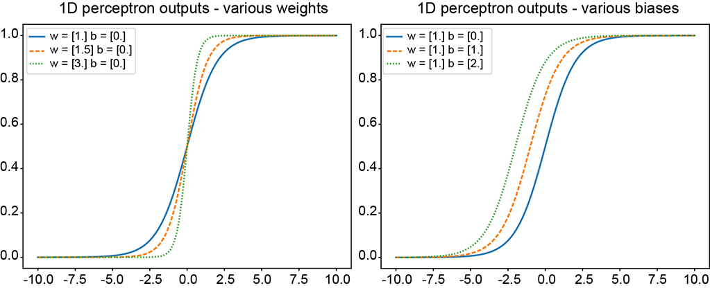
Figure 8.2 Sigmoid curves corresponding to various parameter values in equation 8.2
Some properties of the sigmoid function
The sigmoid function has several interesting properties, some of which are listed here with proof outlines.
-
Expression with positive x:
![]()
Equation 8.3
This expression can be easily proved by multiplying both the numerator and denominator of equation 1.5 by ex.
-
Sigmoid of negative x:
![]()
Equation 8.4
-
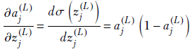
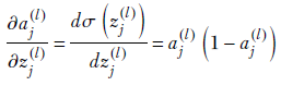
Derivative of sigmoid:

Equation 8.5
Figure 8.3 shows the graph of the derivative of the sigmoid superimposed on the sigmoid graph itself. As expected, the derivative has its maximum value at the middle of the sigmoid curve (where the sigmoid is climbing more or less linearly) and is near zero at both ends (where the sigmoid is saturated and flat, hardly changing).
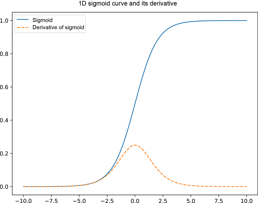
Figure 8.3 Graph of a 1D sigmoid function (solid curve) and its derivative (dashed curve)
8.1.2 Tanh function
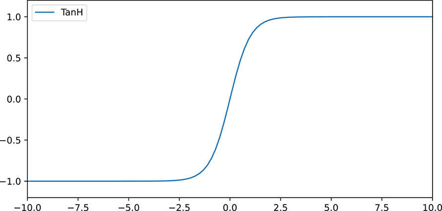
Figure 8.4 Graph of a 1D tanh function.
An alternative to the sigmoid function is the hyperbolic tangent tanh function, shown in figure 8.4. It is very similar to the sigmoid function, but the range of output values is from [−1,1] as opposed to [0,1]. In essence, it is the sigmoid function stretched and shifted so it is centered around 0. The equation of the tanh function is given by
![]()
Equation 8.6
Why is tanh preferred over sigmoid? To understand this, consider figure 8.5. It compares the derivatives of the sigmoid and tanh functions. As the plot shows, the derivative (gradient) of the function near x = 0 is much higher for tanh than for sigmoid. Stronger gradients mean faster convergence, as the weight updates happen in larger steps. Note that this holds mainly when the data is centered around 0: in most preprocessing steps, we standardize the data (make it 0 mean) before feeding it into the neural network.
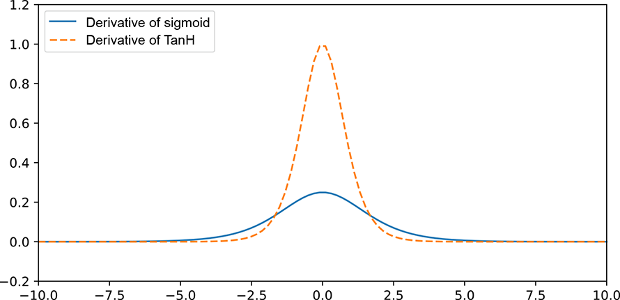
Figure 8.5 Graph of the derivatives of 1D sigmoid and tanh functions
8.2 Why layering?
In section 7.5, we encountered the idea of layering as the preferred way to organize multiple perceptrons. The main property of a layered network is that neurons in any layer take their input only from the outputs of the preceding layer. This means connections exist only between successive layers. No other connection exists in the MLP, which greatly simplifies the evaluation and training of the network, which will become apparent as we discuss forward propagation and backpropagation.
Why have layers at all? We have seen that multiple perceptrons allow us to model problems that cannot be solved by a single perceptron (such as the XOR problem discussed in section 7.4.1). In theory, it is possible to model all mathematical functions (and hence solve all quantifiable problems) with neurons organized in a single hidden layer (see Cybenko’s theorem and proof in section 7.5.3). However, that does not mean a single hidden layer is the most efficient way of doing all modelings. We can often model complicated problems with fewer perceptrons if we organize them in more than one layer.
Why do extra layers help? The primary reason is the extra nonlinearity. Each layer brings in its own nonlinear (such as sigmoid) function. Nonlinear functions, with proper parametrization, can model more complicated functions. Hence, a larger count of nonlinear functions in the model typically implies greater expressive power.
8.3 Linear layers
Various types of layers are used in popular neural network architectures. In subsequent chapters, we shall look at different kinds of layers, such as convolution layers. But in this section, we examine the simplest and most basic type of layer: the linear layer. Here every perceptron from the previous layer is connected to every perceptron in the next layer. Such a layer is also known as fully connected layer. Thus if the previous layer has m neurons and the next layer has n neurons, there are mn connections, each with its own weight.
NOTE We use the words neuron and perceptron interchangeably.
Figure 8.6 shows a linear layer that is a slice of a bigger MLP. Figure 8.7 shows a bigger MLP with a linear layer. Consistent with previous chapters, we have used superscripts for layer IDs and subscripts for source and destination IDs.
The weight of the connection from the kth neuron in layer (l − 1) to the jth neuron in layer l is denoted wjk(l). Here the subscript ordering is the destination (j) followed by the source (k). This is slightly counterintuitive but universally followed because it simplifies the matrix notation (described shortly). Note the following:
-
We have split a single perceptron (weighted sum followed by sigmoid) into two separate layers, weighted sum and sigmoid.
-
We have used sigmoid instead of Heaviside as the nonlinear function.
8.3.1 Linear layers expressed as matrix-vector multiplication
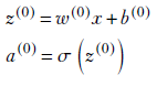
Let’s revisit the perceptron in the context of the MLP. As we saw in equation 7.3, a single perceptron takes a weighted sum of its inputs and then performs a step function on the result. In an MLP, the inputs to any perceptron in the lth layer come from the previous layer: the (l − 1)th layer.
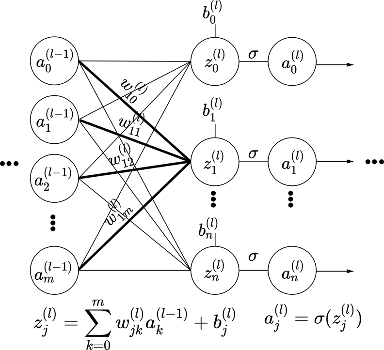
Figure 8.6 Linear layer outputting layer l from layer (l − 1). The weights belonging to row 1 of the weight matrix (coming from all the input neurons, layer (l − 1), which sum together to form output neuron 1) are shown in bold.
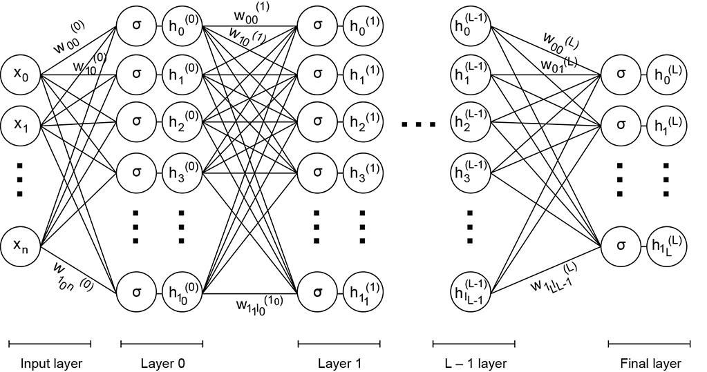
Figure 8.7 Multilayered neural networks: This is a complete deep neural network, a slice of which is shown in figure 8.6.
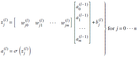
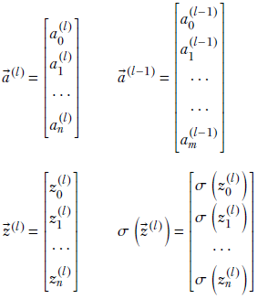
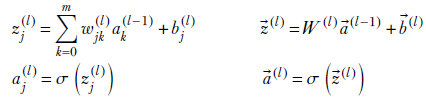
Let a0(l − 1), a1(l − 1), ⋯, am(l − 1) denote the outputs of the m neurons in layer (l − 1) (the left-most input column of nodes in figure 8.6). And let a0(l), a1(l), ⋯, an(l) denote the outputs of the n neurons in layer l. Note that we typically use the symbol a, standing for activation, to denote the output of individual neurons. Now consider the jth neuron in layer l. For instance, check z1(l) in figure 8.6: note the weights going into it and the activations at their source. Its output is aj(l), where
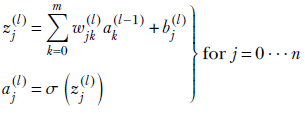
We can rewrite the summation in these equations as a dot product between the weight and activation vectors:
The complete set of equations for all js together can be written in a super-compact way using matrix-vector multiplication,
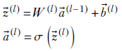
Equation 8.7
where
-
W(l) is an n × m matrix representing the weights of all connections from layer l − 1 to layer l:
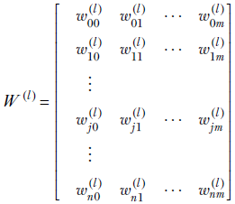
Equation 8.8
-
 (l) represents the activations for the entire layer l. Applying the sigmoid function to a vector is equivalent to applying it individually to each element of the vector:
The matrix-vector notation saves us from dealing with subscripts by working with all the weights, biases, activations, and so on in a global fashion.
8.3.2 Forward propagation and grand output functions for an MLP of linear layers
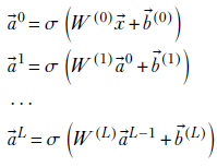
Equation 8.7 describes the forward propagation of a single linear layer. The final output of an MLP with fully connected (aka linear) layers 0⋯L on input ![]() can be obtained by repeated application of this equation:
can be obtained by repeated application of this equation:
MLP(![]() ) =
) = ![]() (L) = y = σ(W(L)…σ(W(1)σ(W(0)
(L) = y = σ(W(L)…σ(W(1)σ(W(0)![]() +
+ ![]() (0))+
(0))+![]() (1))⋯+
(1))⋯+![]() (L))
(L))
Equation 8.9
In a computer implementation, this expression is evaluated step by step by repeated application of the linear layer:
Equation 8.10
It’s easy to see that equation 8.10 is a restatement of equation 8.7.
Close examination of these equations reveals a beautiful property. The complicated equation 8.9 is never explicitly evaluated. Instead, we evaluate the outputs of successive layers, one layer at a time, as per equation 8.10. Every layer can be evaluated by taking the previous layer’s output as input. No other input is necessary. That is to say, we can evaluate ![]() (0) directly from the input
(0) directly from the input ![]() , then
, then ![]() (1) from
(1) from ![]() (0),
(0), ![]() (2) from
(2) from ![]() (1), and so forth, all the way to
(1), and so forth, all the way to ![]() (L) (which is the grand output of the MLP). During the evaluation, we need to keep only the previous and current layers in memory at any given time. This process greatly simplifies the implementation as well as the conceptualization and is known as forward propagation.
(L) (which is the grand output of the MLP). During the evaluation, we need to keep only the previous and current layers in memory at any given time. This process greatly simplifies the implementation as well as the conceptualization and is known as forward propagation.
Listing 8.1 PyTorch code for forward propagation
def Z(x, W_l, b_l):                    ①
    return torch.matmul(W_l, x) + b_l

def A(z_l):                            ②
    return torch.sigmoid(z_l)


def forward(x, W, b):                  ③
    L = len(W) - 1
    a_l = x
    for l in range(0, L + 1):          ④
        z_l = Z(a_l, W[l], b[l])       ⑤
        a_l = A(z_l)                   ⑥
    return a_l
① x: activation of layer l-1 (1-d vector) Wl: Weight matrix of layer l bl: Bias vector of layer l
② Sigmoid activation function (nonlinear layer)
③ x: 1-d input vector W: list of matrices for layers 0 to L. b: list of vectors for layers 0 to L
④ Loops through layers 0 to L
⑤ Computes Z
⑥ Computes activation
8.4 Training and backpropagation
Throughout the book, we have been discussing bits and pieces of this process. In sections 1.1 and 3.3 (specifically, algorithm 3.1 ), we saw an overview of the process for training a supervised model (you are encouraged to reread those if necessary). Training is an iterative process by which the parameters of the neural network are estimated. The goal is to estimate the parameters (weights and biases) such that on the training inputs, the neural network outputs are close as possible to the known ground-truth outputs.
In general, iterative processes improve (get closer to the goal) gradually. In each iteration, we make small adjustments to the parameters. Here, parameter refers to the weights and biases of the MLP, the wjk(l)s and bj(l)s from section 8.2. We keep adjusting the parameters so that in every iteration, the outputs on training data inputs come a little closer to the ground truth (GT). Eventually, after many iterations, we hopefully converge to optimal values. Note that there is no guarantee that the iterative process will converge to the best possible parameter values. The training might go completely astray or get stuck in a local minimum. (Local minima are explained in section 3.6; you are encouraged to reread it if necessary.) There is no good way to know whether we have reached optimal values (global minima) for the weights and biases. We typically run the neural network on test data, and if the results are satisfactory, we stop training. Test data should be held back during training, meaning we should never use test data to train. In the unfortunate event that the network has not reached the desired level of accuracy, we typically throw in more training data and/or try a modified loss function and/or a different architecture. Simply retraining the network from a different random start may also work. This is an experimental science with a lot of trial and error.
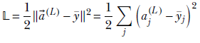
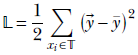
How do we know how to adjust the parameter values in each iteration? We define a loss (aka error) function. There are many popular formulations of loss functions, and we review many of them later, but their common property is that when the neural network output agrees more with the known output (GT), the loss becomes lower, and vice versa. Thus if y denotes the output of the neural network and ȳ is the GT, a reasonable expression for the loss is the mean squared error (MSE) function (y − ȳ)2. For now, we use the MSE loss as our representative loss function. Later we discuss others.
Once the loss function is defined, we have a crisp, quantitative definition of the goal of neural network training. The goal is to minimize the total loss over the entire training data set. Note the clause entire training data set: we do not want to do well on one or two input instances at the cost of doing badly over the rest. If we have to choose between a solution that gives 10% error on all of, say, 100 training input instances versus one that yields 0% error on 50 training input instances but 40% on the remaining 50, we prefer the former.
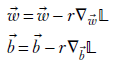
Each weight in the MLP, wjk(l), is adjusted by an amount proportional to δwjk(l). Similarly, each bias bj(l) is adjusted by an amount proportional to δbj(l). We can denote all this compactly by saying we have a weight vector ![]() and bias vector
and bias vector ![]() . In each iteration, we change
. In each iteration, we change ![]() by amount δ
by amount δ![]() and
and ![]() by δ
by δ![]() so that their new values are
so that their new values are ![]() − rδ
− rδ![]() and
and ![]() − rδ
− rδ![]() r is a constant known as the learning rate that needs to be set at the beginning of training). In this context, it is worthwhile to note that in section 8.3.1, we expressed the collection of weights in an MLP with a matrix, while here we are referring to the same thing as a vector. These are not incompatible because we can always rasterize the elements of a matrix (that is, walk over the elements of the matrix from top to bottom and from left to right) into a vector.
r is a constant known as the learning rate that needs to be set at the beginning of training). In this context, it is worthwhile to note that in section 8.3.1, we expressed the collection of weights in an MLP with a matrix, while here we are referring to the same thing as a vector. These are not incompatible because we can always rasterize the elements of a matrix (that is, walk over the elements of the matrix from top to bottom and from left to right) into a vector.
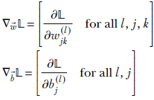
How do we estimate the adjustment amounts δ![]() and δ
and δ![]() ? This is where the notion of gradients comes in. These were discussed in detail in sections 3.3.1, 3.3.2, and 3.5 (again, you are encouraged to reread if necessary). In general, if a loss, denoted 𝕃, is expressed as a function of the parameters, such as 𝕃(
? This is where the notion of gradients comes in. These were discussed in detail in sections 3.3.1, 3.3.2, and 3.5 (again, you are encouraged to reread if necessary). In general, if a loss, denoted 𝕃, is expressed as a function of the parameters, such as 𝕃(![]() ,
, ![]() ), then the change in the parameters that optimally takes us toward lower loss is yielded by the gradient of the loss with respect to the parameters ∇
), then the change in the parameters that optimally takes us toward lower loss is yielded by the gradient of the loss with respect to the parameters ∇![]() , b𝕃(
, b𝕃(![]() , b). The high-level process is described later in the chapter in algorithm 3.2. Here we look at the guts of it.
, b). The high-level process is described later in the chapter in algorithm 3.2. Here we look at the guts of it.
8.4.1 Loss and its minimization: Goal of training
Given a training data set 𝕋 that is a set of <input, GT output> pairs 𝕋 = {⟨![]() , ȳ⟩}, the loss can be expressed as
, ȳ⟩}, the loss can be expressed as
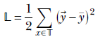
Equation 8.11
where
![]() = MLP(
= MLP(![]() )
)
as per equation 8.9.
Now consider equation 8.7 again. We can rasterize each layer’s weight matrix W(l) into a vector and then concatenate all these vectors from successive layers to form a giant weight vector ![]() , the vector of all weights in the MLP:
, the vector of all weights in the MLP:
![]()
Similarly, we can form a giant vector of all biases in the MLP:
![]()
The ultimate goal of training is to find ![]() and
and ![]() that will minimize the loss 𝕃. In chapter 3, we saw that we can solve for the minimum by setting the gradients ∇
that will minimize the loss 𝕃. In chapter 3, we saw that we can solve for the minimum by setting the gradients ∇![]() 𝕃 = 0 and ∇
𝕃 = 0 and ∇![]() 𝕃 = 0. Computing the loss gradient from a combination of equations 8.9 and 8.11 is intractable. Instead, we go for an iterative solution: gradient descent on the loss surface, as described in the next section.
𝕃 = 0. Computing the loss gradient from a combination of equations 8.9 and 8.11 is intractable. Instead, we go for an iterative solution: gradient descent on the loss surface, as described in the next section.
Listing 8.2 PyTorch code for MSE loss
def mse_loss(a_L, y):                      ①
    return 1./ 2 * torch.pow((a_L - y), 2) ②
① a: Activation of layer L (1D vector) : Ground truth (1D vector)
② See equation 8.11.
8.4.2 Loss surface and gradient descent
Geometrically, the loss function 𝕃(![]() ,
, ![]() ) can be viewed as a surface in a high-dimensional space. The domain of this space corresponds to all the dimensions in
) can be viewed as a surface in a high-dimensional space. The domain of this space corresponds to all the dimensions in ![]() plus all the dimensions in
plus all the dimensions in ![]() . This is shown in figure 8.8 with a 2D domain. In chapter 3, we also saw that given a function 𝕃(
. This is shown in figure 8.8 with a 2D domain. In chapter 3, we also saw that given a function 𝕃(![]() ,
, ![]() ), the best way to progress toward the minimum is to walk on the parameter space along the negative gradient. We adopt this approach to minimize the loss. We compute the gradients of the loss function with respect to weights and biases and update the weights and bias vectors by an amount proportional to the (negative) of these gradients. Doing this repeatedly takes us close to the minimum. In figure 8.8, the gradient descent path is shown with solid arrows, while an arbitrary non-optimal path to the minimum is shown with dashed arrows.
), the best way to progress toward the minimum is to walk on the parameter space along the negative gradient. We adopt this approach to minimize the loss. We compute the gradients of the loss function with respect to weights and biases and update the weights and bias vectors by an amount proportional to the (negative) of these gradients. Doing this repeatedly takes us close to the minimum. In figure 8.8, the gradient descent path is shown with solid arrows, while an arbitrary non-optimal path to the minimum is shown with dashed arrows.
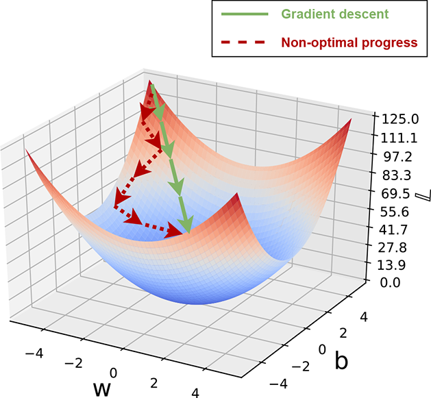
Figure 8.8 A representative loss 𝕃(w, b). Note that ![]() and
and ![]() have each been reduced to 1D for this .
have each been reduced to 1D for this .
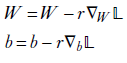
Thus the equations for updating weights and biases in gradient descent are
Equation 8.12
where r is a constant. Here
Equation 8.13
The vector update equation 8.12 can be expressed in terms of the scalar components as
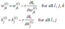
Equation 8.14
Note that we have to reevaluate these partial derivatives in each iteration since their values will change in every iteration.
8.4.3 Why a gradient provides the best direction for descent
Why does updating along the gradient reduce the function optimally? This is discussed in detail in chapter 3. Here we briefly recap the idea. Using multidimensional Taylor expansion, we can evaluate a function in the neighborhood of a known point. For instance, we can evaluate 𝕃(![]() + δ
+ δ![]() ) for small offset δ
) for small offset δ![]() from
from ![]() as follows
as follows
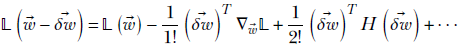
Equation 8.15
where H, called the Hessian matrix, is defined as in equation 3.9. Since we are not going too far from ![]() , ||δ
, ||δ![]() || is small. This means the quadratic and higher-order terms are negligibly small, and we can drop them (the approximation is perfect in the limit when ||δ
|| is small. This means the quadratic and higher-order terms are negligibly small, and we can drop them (the approximation is perfect in the limit when ||δ![]() || → 0):
|| → 0):
![]()
But we know the dot product (![]() )T ▽
)T ▽![]() 𝕃 will attain its maximum value when both the vectors point in the same direction: that is,
𝕃 will attain its maximum value when both the vectors point in the same direction: that is,
![]()
for some constant of proportionality r.
In implementation, r is called the learning rate. A higher learning rate causes the optimization to progress more rapidly but also runs the risk of overshooting the minimum. We learn about these in more detail later. For now, simply note that r is a tunable hyperparameter of the system.
Thus, the largest decrease in value from 𝕃(![]() ) to 𝕃(
) to 𝕃(![]() –
– ![]() ) happens when δ
) happens when δ![]() is along the negative gradient. This is why we move toward the negative gradient in gradient descent: it is the fastest way to reach the minimum. The straight arrows in figure 8.8 illustrate the direction of the gradient. The dashed arrows show an arbitrary nongradient path for comparison.
is along the negative gradient. This is why we move toward the negative gradient in gradient descent: it is the fastest way to reach the minimum. The straight arrows in figure 8.8 illustrate the direction of the gradient. The dashed arrows show an arbitrary nongradient path for comparison.
We can deal with the bias vector ![]() similarly.
similarly.
8.4.4 Gradient descent and local minima
We should note that gradient descent can get stuck in a local minimum. Figure 8.9 shows this.
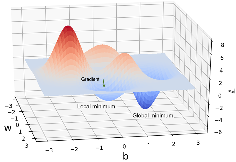
Figure 8.9 A nonconvex function with local and global minima. Depending on the point, gradient descent will take us to one or the other.
In earlier eras, optimization techniques tried hard to avoid local minima and converge to the global minimum. Techniques like simulated annealing and tunneling were carefully designed to avoid local minima. Modern-day neural networks have adopted a different attitude: they do not try very hard to avoid local minima. Sometimes a local minimum is an acceptable (accurate enough) solution. Otherwise, we can retrain the neural network: it will start from a random position, so this time it may go to a better minimum.
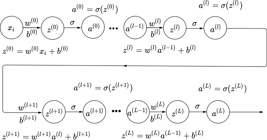
Figure 8.10 MLP with layers 0, …, L, one neuron per layer. Again, we have split every layer into a weighted sum and a sigmoid.
8.4.5 The backpropagation algorithm
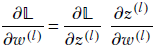
We have seen that gradient descent progresses by repeatedly updating the weights and biases via equation 8.12. This is equivalent to repeatedly updating individual weights and biases using individual partial derivatives via equation 8.14.
Obtaining a closed-form solution for the gradients ∇![]() 𝕃(
𝕃(![]() ,
, ![]() ), ∇
), ∇![]() 𝕃(
𝕃(![]() ,
, ![]() ) from equations 8.9 and 8.11—or, equivalently, obtaining a closed-form solution for the partial derivatives ∂𝕃/∂wjk(l), ∂𝕃/∂bj(l), —is very difficult. Backpropagation is an algorithm that allows us to evaluate the gradients and update the weights and biases one layer at a time, like forward propagation (equation 8.10).
) from equations 8.9 and 8.11—or, equivalently, obtaining a closed-form solution for the partial derivatives ∂𝕃/∂wjk(l), ∂𝕃/∂bj(l), —is very difficult. Backpropagation is an algorithm that allows us to evaluate the gradients and update the weights and biases one layer at a time, like forward propagation (equation 8.10).
Backpropagation algorithm on a simple network
We first discuss backpropagation on a simple MLP with only a single neuron per layer. The main simplification resulting from this is that individual weights and biases no longer need subscripts, with only one weight and one bias between two successive layers. They still need superscripts to indicate layer IDs, however. Figure 8.10 shows this MLP. We use MSE loss (equation 8.11), but we work on a single input-output pair xi, yi. The total loss (summation over all the training data instances) can easily be derived by repeating the same steps.
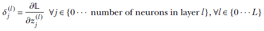
We first define an auxiliary variable:
![]()
The physical significance of δ(l) is that it is the rate of change of the loss with the (pre-activation) output of layer l (remember, in this network, layer l has a single neuron).
Let’s establish a few important equations for the MLP in figure 8.10:
-
Forward propagation for an arbitrary layer l ∈ {0, L}
![]()
Equation 8.16
![]()
Equation 8.17
-
Loss—Here we are working with a single training data instance, xi, whose GT output is ȳi:
![]()
-
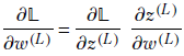
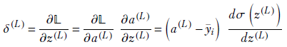
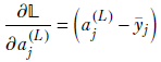
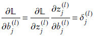
Partial derivative of loss with respect to the weight and bias in terms of an auxiliary variable for the last layer, L—Using the chain rule for partial derivatives,
Examining the terms on the right, we see
![]()
(auxiliary variable for layer L). And using the forward propagation equations,
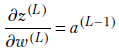
Together, they lead to
![]()
Similarly,
![]()
Consequently, we have the following pair of equations expressing the partial derivative of loss with respect to weight and bias, respectively, in terms of the auxiliary variable for the last layer:
![]()
Equation 8.18
![]()
Equation 8.19
-
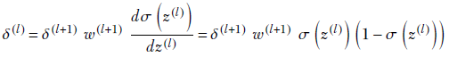
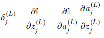
Auxiliary variable for the last layer, L—Using the chain rule for partial derivatives,
Using equation 8.5 for the derivative of a sigmoid, we get
δ(L) = (a(L)−ȳi) σ(z(L))(1−σ(z(L)))
which, using equation 8.17, leads to
δ(L) = (a(L)−ȳi) a(L)(1−a(L))
Equation 8.20
-
Partial derivative of the loss with respect to the weight and bias in terms of an auxiliary variable for an arbitrary layer l—Using the chain rule for partial derivatives,
Using the definition of the auxiliary variable and the forward propagation equation 8.16, this leads to
![]()
Equation 8.21
Similarly,
![]()
Using the definition of the auxiliary variable and the forward propagation equation 8.16, this leads to
![]()
Equation 8.22
-
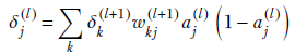
Auxiliary variable for an arbitrary layer, l—Using the chain rule for partial derivatives,
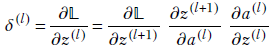
Using the definition of the auxiliary variable and the forward propagation equation 8.16, this leads to
which yields
δ(l) = δ(l+1) w(l+1) a(l)(1−a(l))
Equation 8.23
We first encountered the one-layer-at-a-time property in section 8.3.2 in connection with the forward propagation equations. Let’s recap that in the context of training our simple network. Consider equations 8.16 and 8.17. We initialize the system with some values of weights w(l) and biases b(l). Using those, we can evaluate the layer 0 outputs. For starters, we can evaluate z(0) and a(0) easily (since all the inputs are known):
Once we have z(0) and a(0), we can use them to evaluate z(1) and a(1) via equations 8.16 and 8.17. But if we have z(1) and a(1), we can use them to evaluate z(2) and a(2) via equations 8.16 and 8.17 again. And we can proceed in this fashion up to layer L to obtain a(L), which is the grand output of the MLP. In other words, we can iteratively evaluate the outputs of successive layers using only the outputs from the previous layer. No other layers need to be known. At any given iteration, we only have to keep the previous layer in memory: we can build the current layer from that. A single sequence of applications of equations 8.16 and 8.17 for layers 0 to L is known as a forward pass.
A similar trick can be applied to evaluate the auxiliary variables, except we go backward. We can evaluate the auxiliary variable for the last layer, δ(L), via equation 8.20. But once we have δ(L), we can evaluate δ(L − 1) via equation 8.23. From that, we can evaluate δ(L − 2). We can proceed in this fashion all the way to layer 0, evaluating successively δ(L), δ(L − 1), ⋯, δ(0). Every time we evaluate a δ(l), we can also evaluate the ∂𝕃/∂w(l) and ∂𝕃/∂b(l) for the same layer via equations 8.21 and 8.22, respectively. We can also update the weight and bias of that layer right there using the just estimated partial derivatives, since the current values will never be needed again during training. Thus, starting from the last layer, we can update the weights and biases of all layers until layer 0 in this fashion. This is backpropagation.
Of course, we have to proceed in tandem: one forward propagation which sets the values of zs and as) for layers 0 to L, followed by a backpropagation layer for L to 0. Repeat these steps until convergence.
NOTE Fully functional code for forward propagation, MSE loss, and backpropagation, executable via Jupyter Notebook, can be found at http://mng.bz/pJrw.
Listing 8.3 PyTorch code for forward and backward propagation
def forward_backward(x, y, W, b):
    L = len(W) - 1
    a = []
    for l in range(0, L+1):
        a_prev = x if l == 0 else a[l-1]              ①
        z_l = Z(a_prev, W[l], b[l])
        a_l = A(z_l)
        a.append(a_l)

    loss = mse_loss(a[L], y)                          ②

    deltas = [None for _ in range(L + 1)]
    W_grads = [None for _ in range(L + 1)]            ③
    b_grads = [None for _ in range(L + 1)]

    a_L = a[L]                                        ④
    deltas[L] = (a_L - y) * a_L * (1 - a_L)
    W_grads[L] = torch.matmul(deltas[L], a[L - 1].T)  ⑤
    b_grads[L] = deltas[L]

    for l in range(L-1, -1, -1):                      ⑥
        a_l = a[l]
        deltas[l] =  torch.matmul(W[l+1].T, deltas[l + 1]) * a_l * (1 - a_l)
        W_grads[l] = torch.matmul(deltas[l], a[l - 1].T)
        b_grads[l] = deltas[l]

    return loss, W_grads, b_grads
① Forward propagation
② Computes MSE loss
③ Arrays to store δ(l), ∂𝕃/∂w(l), ∂𝕃/∂b(l) for layers 0 to L
④ Activation of the last layer - a(L)
⑤ Computes the δ and gradients for layer L
⑥ Computes the δ and gradients for layers 0 to L − 1
Backpropagation algorithm on an arbitrary network of linear layers
In section 8.4.5.1, we saw a simple network with only one neuron per layer. There was only one connection and hence one weight, one activation, and one auxiliary variable per layer. Consequently, we could drop the subscripts (although we had to keep the superscript indicating the layer) of all these variables. Now we examine a more generic network consisting of linear layers 0, ⋯, L. An arbitrary slice of this network is shown in figure 8.6.
The ultimate goal is to evaluate the partial derivatives of the loss with respect to the weights and biases. Using them, we can update the current weights and biases to optimally reduce the loss.
Our overall strategy is as follows. We use the auxiliary variables again. We first derive expressions that allow us to compute the auxiliary variable for the last layer. Then we derive an expression that allows us to compute auxiliary variables for an arbitrary layer, l, given the auxiliary variables for layer l + 1. Since we can directly compute auxiliary variables for the last layer, L, we can use this expression to compute auxiliary variables for the second-to-last layer L − 1. But once we have them, we can compute auxiliary variables for layer L − 2. We proceed like this until we reach layer 0. Thus we can compute all the auxiliary variables. We also derive expressions that allow us to compute, from the auxiliary variables, the partial derivatives of loss with respect to weights and biases. This gives us everything we need. Since we start by computing things pertaining to the last layer and proceed iteratively toward the initial layer, the process is called backpropagation.
You will notice the similarity between the expressions derived next and those derived for the one-neuron-per-layer network. The differences are explained:
-
Forward propagation (arbitrary layer l)—Forward propagation through this network has already been described in section 8.3.1 and can be succinctly represented by equation 8.7 repeated here for handy reference). On the left are the scalar equations, for one neuron at a time; and on the right are the vector equations, for the entire layer. They are equivalent:
Equation 8.24
Indices j and k iterate over all the neurons in the relevant layer. By convention, we always use these variables for arbitrary neurons in a layer. The variable l is used to index the layers. When indexing weights, we typically use j to indicate the destination and k to indicate the source—remember that weights are indexed (destination, source) somewhat unexpectedly to simplify the math. Typically, vectors correspond to entire layers. Individual vector elements correspond to specific neurons and are indexed by j or k.
-
Loss—Unlike the simple network, here, the final Lth layer can have multiple neurons. Hence the loss function becomes
Equation 8.25
where the summation happens over all neurons in the last layer. Note that ![]() (L) is the output of the MLP: that is,
(L) is the output of the MLP: that is, ![]() (L) =
(L) = ![]() = MLP(
= MLP(![]() ) for the training input
) for the training input ![]() (see equation 8.10). The GT output corresponding to
(see equation 8.10). The GT output corresponding to ![]() is the constant vector ȳ. The closer
is the constant vector ȳ. The closer ![]() is to ȳ, the smaller the loss. Note that we need to average the loss over the entire training data set. Here we are showing the loss computation for a single training data instance. The computation simply needs to be replicated for each training data instance, and the results averaged.
is to ȳ, the smaller the loss. Note that we need to average the loss over the entire training data set. Here we are showing the loss computation for a single training data instance. The computation simply needs to be replicated for each training data instance, and the results averaged.
-
Auxiliary variables—Now that a layer has multiple neurons, we have one auxiliary variable per neuron. Thus the auxiliary variable has a subscript identifying the specific neuron in that layer. It continues to have a superscript indicating its layer. We define
-
Auxiliary variable for the last layer
Using equation 8.25 and observing that only one of the terms in the summation—the jth term—will survive the differentiation with respect to aj(L) since the ajs are independent of each other), we get
Also, using the lower-left equation from 8.24 and equation 8.5, we get
Combining these, we get
![]()
Equation 8.26
![]()
Equation 8.27
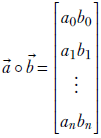
Here, ∘ denotes the Hadamard product between two vectors. It is basically a vector of elementwise products of corresponding vector elements. Thus,
Equation 8.28
Equation 8.29
Equations 8.26 and 8.27 are identical. The former is a scalar equation expressing individual auxiliary variables of the last layer. The latter is a vector equation expressing all the auxiliary variables of the last layer together. We can compute these directly if we have performed a forward pass and have its results, the aj(L)s available along with the training data GT.
-
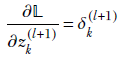
Auxiliary variable for an arbitrary layer, l—This is significantly different and harder to understand than the one-neuron-per-layer case. We are trying to evaluate δj(l) = ∂𝕃/∂zj(l) in the general case: that is, for an arbitrary layer l. The loss does not directly depend on the inner layer variable zj(l). The loss directly depends only on the last layer activations, which depend on the previous layer, and so forth. The zs in any one layer form a complete dependency set for the loss 𝕃, meaning the loss can be expressed in terms of only these and no other variables. In particular, we can express the loss as 𝕃(z0(l+1), z1(l+1), z2(l+1),⋯). You can form a mental picture that zj(l) fans out to 𝕃 through all the zs in the next layer, z0(l+1), z1(l+1), z2(l+1), and so on. Then, using the chain rule of partial differentiation,
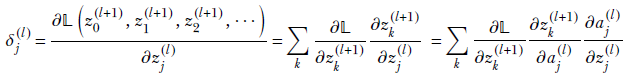
Now, by definition,
And using equation 8.24,
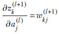
while
Combining all these, we get the scalar expression for a single auxiliary variable. It is presented here along with its equivalent vector equation for the entire layer:
Equation 8.30
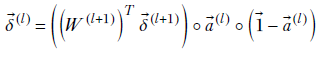
Equation 8.31
Here, ∘ denotes the Hadamard multiplication explained earlier and W(+1l) is the matrix representing the weights of all connections from layer l to layer (l+1) (see equation 8.8). Equations 8.30 and 8.31 allow us to evaluate δ(l)s from the δ(l+1)s if the results of forward propagation (as) are available. We have already shown that the auxiliary variables for the last layer are directly computable from the activations of that layer. Hence, we can evaluate all the layers’ auxiliary variables.
-
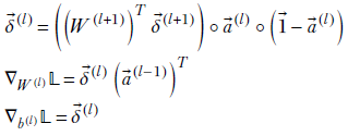
Derivatives of loss with respect to weights and biases in terms of auxiliary variables—We have already seen how to compute auxiliary variables. Now we will express the partial derivatives of loss with respect to weights and biases in terms of those. This will provide us with the gradients we need to update the weights and biases along the negative gradient, which is the optimal move to minimize loss:
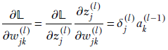
Equation 8.32
![]()
Equation 8.33
Equations 8.32 and 8.33 are equivalent. The first is scalar and pertains to individual weights in layer l, and the second describes the entire layer. Similarly, equations 8.34 and 8.35 are equivalent:
Equation 8.34
![]()
Equation 8.35
The first is scalar and pertains to individual biases in layer l, and the second describes the entire layer.
8.4.6 Putting it all together: Overall training algorithm
Previously, we discussed forward propagation: passing an input vector ![]() through a sequence of linear layers and generating an output prediction. We learned about MSE loss, 𝕃, which calculates the deviation of the output prediction from the GT, y. We also learned to compute the gradients of 𝕃 with respect to parameters W and b using backpropagation. In the following algorithm, we describe how these components come together in the training process:
through a sequence of linear layers and generating an output prediction. We learned about MSE loss, 𝕃, which calculates the deviation of the output prediction from the GT, y. We also learned to compute the gradients of 𝕃 with respect to parameters W and b using backpropagation. In the following algorithm, we describe how these components come together in the training process:
Algorithm 8.5 Training a neural network
Initialize ![]() , b with random values
, b with random values
while 𝕃 > threshold do
⊳ Forward pass
for l ← 0 to L do
![]() (l) = W(l)
(l) = W(l) ![]() (l–1) +
(l–1) + ![]() (l)
(l)
![]() (l) = σ(
(l) = σ(![]() (l))
(l))
end for
⊳ Loss
𝕃 = 1/2 ||![]() (L) – ȳ||2
(L) – ȳ||2
⊳ Gradients for the last layer
![]() (L) = (
(L) = (![]() (L) – ȳ) ∘
(L) – ȳ) ∘ ![]() (L) ∘ (
(L) ∘ (![]() –
– ![]() (L))
(L))
▽W(L)𝕃 = ![]() (L)(
(L)(![]() (L–1))T
(L–1))T
▽b(L)𝕃 = ![]() (L)
(L)
⊳ Gradients for the remaining layers
for l ← L – 1 to 0 do
![]() (l) = ((W(l+1))T
(l) = ((W(l+1))T ![]() (l+1))
(l+1)) ![]() (l) ∘ (
(l) ∘ (![]() –
– ![]() (l))
(l))
▽W(l)𝕃 = ![]() (l) (
(l) (![]() (l–1))T
(l–1))T
▽b(l)𝕃 = ![]() (l)
(l)
end for
⊳ Parameter update
W = W – r▽W𝕃
b = b – r▽b𝕃
end while
8.5 Training a neural network in PyTorch
Now that we’ve seen how the training process works, let’s look at how this can be implemented in PyTorch. For this purpose, let’s take the following example. Consider an e-commerce company that’s trying to solve the problem of demand prediction: the company would like to estimate the number of mobile phones that will be sold in the upcoming week so that it can manage its inventory accordingly. Our goal is to develop a model that can make such a prediction. Let’s assume that the demand for a given week is a function of three variables: (a) the number of mobile phones sold in the previous week, (b) discounts offered, and (c) the number of weeks to the next holiday. Let’s call these variables prev_week_sales, discount_fraction, and weeks_to_next_holidays, respectively. This example can be modeled as a regression problem wherein we predict the number of mobile phones sold in the upcoming week from an input vector of the form [prev_week_sales, discount_fraction, weeks_to_next_holidays].
NOTE Fully functional code for this section, executable via Jupyter Notebook, can be found at http://mng.bz/O1Ra.
From historical data, we generate a large data set, X, that contains the values of the three variables for the last N weeks. X is represented as an N x 3 matrix, with each row representing an individual training data instance and N being the total number of data points available. We also have a GT vector ȳ of length N, containing the actual sales of mobile phones for each of the weeks in the training data set. Table 8.1 shows sample data points from our training set.
Table 8.1 Sample training data for demand prediction
|
Previous week sales |
Discount fraction (%) |
Weeks to next holidays |
Number of units sold |
|---|---|---|---|
|
76,440 |
63 |
2 |
94,182 |
|
41,512 |
50 |
3 |
51,531 |
|
77,395 |
77 |
9 |
95,938 |
|
… |
… |
… |
… |
|
21,532 |
70 |
4 |
28,559 |
NOTE In this section, X and ȳ refer to the entire batch of training data instances. This may be infeasible in practical settings because of large data sets. To address this, we typically use mini-batches of X and ȳ. We introduce the concept of mini-batches formally in the next chapter.
One important point about the data set is that the range of values for each feature is completely different. For example, the previous week’s sales are expressed as a number on the order of tens of thousands of units, whereas the discount fraction is a percentage number between 0 and 100. In machine learning, it is a good practice to bring all the values to a common scale, because doing so can help improve the speed of training and reduce the chance of getting stuck at a local minimum. For our example, let’s use min-max normalization to scale all the features to 0–1. The following code snippet shows how to perform min-max normalization in PyTorch. For the rest of the discussion, we assume that we are operating on the normalized data:
def min_max_norm(X, y):
    X, y = X.clone(), y.clone()              ①
    X_min, X_max = torch.min(X, dim=0)[0],
            torch.max(X, dim=0)[0]           ②
    X = (X - X_min) / (X_max - X_min)        ③
    y_min, y_max = torch.min(y, dim=0)[0],
            torch.max(y, dim=0)[0]           ④
    y = (y - y_min) / (y_max - y_min)        ⑤
    return X, y
① Clones the data so as not to mutilate the original data
② Calculates the min and max values of each column of X
③ Normalizes X
④ Calculates the min and max values of y
⑤ Normalizes y
To solve the regression problem, let’s first define a two-layer neural network model that can take in 3D input vectors of the form [prev_week_sales, discount_fraction, is_holidays_ongoing] and generate output predictions. The following code snippet gives the PyTorch implementation:
class TwoLayeredNN(torch.nn.Module):
    def __init__(self, input_size, hidden1_size, hidden2_size, output_size):
        super(TwoLayeredNN, self).__init__()

        self.model = torch.nn.Sequential(                  ①

            torch.nn.Linear(input_size, hidden1_size),     ②
            torch.nn.Sigmoid(),

            torch.nn.Linear(hidden1_size, hidden2_size),   ③
            torch.nn.Sigmoid(),

            torch.nn.Linear(hidden2_size, output_size)     ④
        )

    def forward(self, X):                                  ⑤
        return self.model(X)

nn = TwoLayeredNN(input_size=X.shape[-1], hidden1_size=10,
                                  hidden2_size=5, output_size=1)
① Defines the network as a sequence of linear and sigmoid layers
② First hidden layer with a weight matrix of size input_size × hidden1_size)
③ Second hidden layer with a weight matrix of size hidden1_size × hidden2_size)
④ Output layer with a weight matrix of size hidden2_size × output_size)
⑤ X is an N × 3 matrix. Each row is a (3D vector) representing a single data point.
Neural network models in PyTorch should subclass torch.nn.Module and implement the forward method. Our two-layer neural network contains two linear layers, each followed by a sigmoid (nonlinear) activation layer. Finally, we have a linear layer that converts the final activation into the output prediction. These layers are chained together using the torch.nn.Sequential class to form the two-layer neural network. Whenever our model is called using nn(X), the forward method is invoked, and the input X is passed through the individual layers to obtain the final output.
Now that we have defined the neural network and its forward pass, we need to define the loss function. We can use the MSE loss defined in equation 8.11. The loss function essentially compares the demand predicted by the neural network model with the actual demand from the GT and returns larger values when the difference is higher and smaller values when the difference is lower. MSE loss is readily available in PyTorch through the torch.nn.MSELoss class. The following code snippet shows a sample invocation:
loss = torch.nn.MSELoss() ①

loss(y_pred, y_gt)        ②
① Instantiates the loss function
② compute loss _pred: Output of the neural network _gt: ground truth
Finally, we need a way to compute the gradients of the loss with respect to the parameters of our model so we can start the training process. Luckily, we don’t have to explicitly compute the gradients ourselves because PyTorch automatically does this for us using automatic differentiation, aka autograd. (Refer to section 3.1 for more details about autograd.) For our current example, we can instruct PyTorch to run backpropagation and compute gradients by calling loss.backward(). With this, we’re ready to start training. PyTorch code for training the neural network is shown next.
Listing 8.4 Training a neural network
nn = TwoLayeredNN(input_size=X.shape[-1],             ①
                  hidden1_size=10,
                  hidden2_size=5,
                  output_size=1)
loss = torch.nn.MSELoss()                             ②
optimizer = torch.optim.SGD(nn.parameters(), lr=0.2,  ③
                            momentum=0.9)
num_iters = 1000

for i in range(num_iters):                            ④
    y_out = nn(X)                                     ⑤
    mse_loss = loss(y_out, y)                         ⑥
    optimizer.zero_grad()                             ⑦
    mse_loss.backward()                               ⑧
    optimizer.step()                                  ⑨
① Instantiates the neural network
② Instantiates the loss function
③ Instantiates the optimizer
④ Training loop
⑤ Forward pass
⑥ Computes the loss
⑦ Clears the gradients and prevents accumulation of gradients from the previous step
⑧ Runs backpropagation (computes gradients)
⑨ Updates the weights
In the training loop, we iteratively run the forward pass, compute the loss, calculate the gradients, and update the weights. The neural network is initialized with random weights and hence makes arbitrary predictions for the demand in the early iterations of the training loop. This translates to a high initial loss value. However, as training proceeds, the weights are updated to minimize the loss value, and the predicted demand comes closer to the actual GT. To update the weights, we use what is known as an optimizer. During training, the gradients are computed by calling the backward() function on the loss object. Following that, the optimizer.step call updates the weights and biases. In this example, we used the stochastic gradient descent–based optimizer, which can be invoked using torch.optim.SGD. PyTorch offers various optimizers, such as Adam, AdaGrad, and so on, which will be discussed in detail in the next chapter. We typically run the training loop until the loss reaches a value low enough to be acceptable. Once the training loop completes, we have a model that can readily take in new data points and generate output predictions.
Summary
-
The sigmoid function σ(x) = 1/1+e–x has an S-shaped graph, is a differential version of the Heaviside step function, and, as such, is used in perceptrons. Thus the overall perceptron function becomes P(
 ) ≡ σ(
 T + b). It is parametrized by and b, which control the slope and position, respectively, of the S-shaped curve.
 -
Neural networks solve real-life problems that require intelligence by approximating the function that solves the problem in question. They are built of multiple perceptrons interconnected by weighted edges. Instead of connecting perceptrons haphazardly, we connect them as layers. In a layered network, a perceptron is only connected to perceptrons from the immediately preceding layer. Intra-layer and other connections are not allowed.
-
Supervised neural networks have manually generated outputs for a sample set of input values (ground truth). This entire data set consisting of inputs and known outputs is known as the training data set.
-
Loss is defined as the mismatch between the ground truth and actual output generated by the neural network on training data inputs. The simplest way to compute loss is to take the Euclidean distance between the neural network-generated output and ground-truth vectors. This is called the MSE (mean squared error) loss. Mathematically, given a training data set 𝕋 that is a set of <input, GT output> pairs 𝕋 = {⟨
, ȳ⟩}, the loss can be expressed as
where the output is ![]() i = MLP(
i = MLP(![]() i).
i).
-
Training is the process of optimizing the connection weights and biases of a specific neural network so that the loss is minimal. Note that during inferencing, the neural network typically sees data it has never seen during training. Inferencing outputs are good only if the distribution of training inputs roughly matches the overall input distribution.
-
We minimize the loss by iteratively adjusting the weights and biases. The quickest way to reach the closest minimum of a multivariate function is to follow the gradient. Hence, we adjust the weights and biases following the gradient of the loss function. Mathematically,
-
A forward pass is the process of generating outputs from inputs with a neural network: more specifically, a multilayer perceptron MLP). Thus an MLP does inferencing via a forward pass. A beautiful property of a layered network is that we can do a forward pass dealing with one layer at a time, proceeding iteratively from layer 0 (closest to the input) to the output layer. Mathematically,
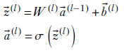
where W(l), ![]() (l) represent the weights and biases for layer l, and
(l) represent the weights and biases for layer l, and ![]() (l) represent the output for layer l activation), which is also the input for layer l + 1.
(l) represent the output for layer l activation), which is also the input for layer l + 1.
-
A backward pass is the process by which the gradients of the loss with respect to all the weights and biases are generated. It relies on the result of the preceding forward pass and proceeds from the output layer toward the input layer. It uses auxiliary variables
 (l), which can be computed by iterating backward from the last (closest to output) layer to the first (closest to input) layer—hence the name backward propagation—and all the required gradients can be computed from those auxiliary variables. Mathematically,