10 Convolutions in neural networks
This chapter covers
- The graphical and algebraic view of neural networks
- Two-dimensional and three-dimensional convolution with custom weights
- Adding convolution layers to a neural network
Image analysis typically involves identifying local patterns. For instance, to do face recognition, we need to analyze local patterns of neighboring pixels corresponding to eyes, noses, and ears. The subject of the photograph may be standing on a beach in front of the ocean, but the big picture involving sand and water is irrelevant.
Convolution is a specialized operation that examines local patterns in an input signal. These operators are typically used to analyze images: that is, the input is a 2D array of pixels. To illustrate this, we examine a few examples of special-purpose convolution operations that detect the edges, corners, and average illumination in a small neighborhood of pixels from an image. Once we have detected such local properties, we can combine them and recognize higher-level patterns like ears, noses, and eyes. We can combine those in turn to detect still higher-level structures like faces. The system naturally lends itself to multilayer convolutional neural
networks—the lowest layers(closest to the input) detect edges and corners, and the next layers detect ears, eyes, noses, and so forth.
In section 8.3, we discussed the linear neural network layer (aka fully connected layer). There, every output is connected to all inputs. This means an output is derived by taking a weighted linear combination of all input values. In other words, the output is derived from a global view of the input. Convolution layers are different. These are characterized by:
-
Local connections—Only a small subset of neighboring input values are connected to one output value. Thus, each output is a weighted linear combination of only a small set of adjacent input values. As a consequence, only local patterns in the input are captured.
-
Shared weights—The same weights are slid over the entire input. Consequently,
-
The number of weights is drastically reduced. Since convolution is typically used on images where the input size is large number of pixels), fully connected layers are prohibitively expensive. Convolution repeats a (usually small) number of weights across the input, thereby keeping the number of weights manageable.
-
The nature of the local pattern extracted is fixed all over the input. If the convolution is an edge detector, it extracts edges all over the input. We cannot have an edge detector at one region of the input and a corner detector at another region, for instance. Of course, in a multilayered network, we can use different convolution layers to capture different local patterns. In particular, successive layers can capture local patterns in local patterns of the input, and so on, thereby capturing increasingly complex and increasingly global patterns at higher layers of the network.
-
The exact local pattern captured depends on the weights of the convolution operator. We don’t know exactly what local patterns of the input to capture to recognize a specific higher-level structure of interest (such as a face). This means we do not want to specify the weights of the convolutions. The whole point of neural networks is to avoid such tailored feature engineering. Rather, we want to learn—through the process of training described in chapter 8—the weights of the convolution layers. Losses can be backpropagated through convolution just as they are through fully connected (FC) layers.
Just like FC layers, convolution layers can be expressed as matrix-vector multiplications. The structure of the weight matrix is a special case of equation 8.8, but it is a matrix all the same. Consequently, the forward propagation equation 8.7 and backpropagation equations 8.31 and 8.33 are still applicable. Forward propagation and backpropagation (training) through convolution proceed exactly as they do with FC layers.
Since the convolution is learned—as opposed to specified—in a neural network, there is no telling what local patterns such layers will learn to extract (although, in practice, the initial layers often learn to recognize edges and corners). All we know is that each output in a given layer is derived from only a small subset of spatially adjoint input values from previous layers. The final output is derived from a hierarchical local examination of the input.
NOTE Fully functional code for chapter 10, runnable via Jupyter Notebook, is available at our public GitHub repository at http://mng.bz/M2lW.
10.1 One-dimensional convolution: Graphical and algebraical view
As always, we examine the process of convolution with a set of examples. We examine convolutions in one, two, and three dimensions, but we start with one dimension for ease of understanding.
The best way to visualize 1D convolution is to imagine a stretched, straightened rope (the input array) over which a measuring ruler (the kernel) is sliding.
-
In figures 10.1, 10.2, and 10.3, the ruler kernel) is shown as shaded boxes, while the rope (input array) is shown as a sequence of white boxes. Successive steps in the figure represent successive positions (aka slide stops) of the sliding ruler. Notice that the shaded portion occupies a different position in each step.
-
Rulers in successive positions during sliding can overlap. They overlap by varying amounts in figures 10.1, 10.2, and 10.3.
-
The rope and the ruler are discrete 1D arrays in reality. At each slide stop, the ruler array elements rest on a subset of rope array elements.
-
We multiply each input array element by the kernel element resting on it and sum the products. This is equivalent to taking a weighted sum of the input (rope) elements that fall under the current position of the kernel (ruler), with the kernel elements serving as weights. This weighted sum is emitted as a single output element. One output element results from each slide stop of the tile. As the ruler slides over the entire rope, left to right, a 1D output array is generated.

Figure 10.1 1D convolution with a local averaging kernel of size 3, stride 1, and valid padding on the input array of size 7
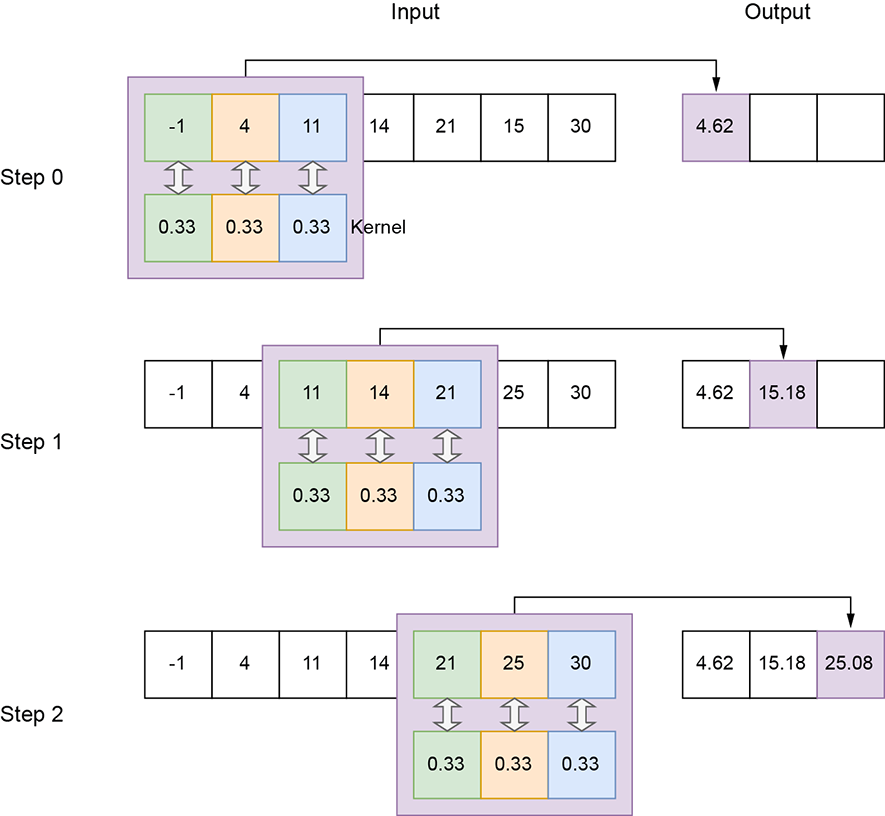
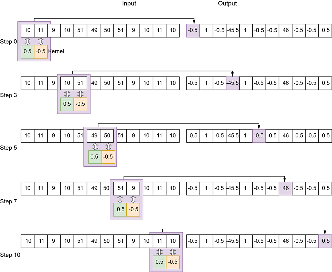
Figure 10.3 1D convolution with an edge-detection kernel of size 2, stride 1, valid padding. Not all slide stops (that is, steps) are shown.
The following entities are defined for 1D convolution:
-
Input—A one-dimensional array. We typically use the symbol n to represent input array length in 1D convolution. In figure 10.1, n = 7.
-
Output—A one-dimensional array. We typically use the symbol o to represent the output array length in 1D convolution. In figure 10.1, o = 5. Section 10.2 shows how to calculate the output size from the independent parameters.
-
Kernel—A small array of weights whose size is a parameter of the convolution. We typically use the symbol k to represent the kernel size in 1D convolution. In figure 10.1, k = 3; in figure 10.3, k = 2.
-
Stride—The number of input elements over which the kernel slides after completing a single step. We typically use the symbol s to represent the stride in 1D convolution. This is a parameter of the convolution. In figure 10.1, s = 1; in figure 10.2, stride is 2. A stride of 1 means there is a slide stop at each successive element of the input. So, the output has roughly the same number of elements as the input (they may not be exactly equal because of padding, explained next). A stride of 2 means there is a slide stop at every other input element. So, the output size is roughly half of the input size. A stride of 3 means the output size is roughly one-third the input size.
-
Padding—As the kernel slides toward the extremity of the input array, parts of it may fall outside the input array. In other words, part of the kernel falls over ghost input elements. Figure 10.4 shows such a situation: the ghost input array elements are shown with dashed boxes. There are multiple strategies to deal with this:
-
Valid padding—We stop sliding whenever any element of the kernel falls outside the input array. No ghost input elements are involved; the entire kernel always falls on valid input elements (hence the name valid). Note that this implies we will have fewer outputs than inputs. If we try to generate an output corresponding to, say, the last input element, all but the first kernel element will fall outside the input on ghost elements. So, we have to stop when the right-most kernel element falls on the right-most input element (see figures 10.1, 10.2, and 10.3). At this point, the left-most kernel element falls on the (N − k)th input element. We do not generate output for the last k inputs. Hence, even with a stride of 1 for valid padding, the output is slightly smaller than the input.
-
Same (zero) padding—Here, we do not want to stop early. If the stride is 1, the output size matches the input size (hence the name same). We continue to slide the kernel until its left end falls on the right-most input. At this point, all but the left-most kernel element is falling on ghost input elements. We pretend these ghost input elements have a value of 0 (zero padding).
-
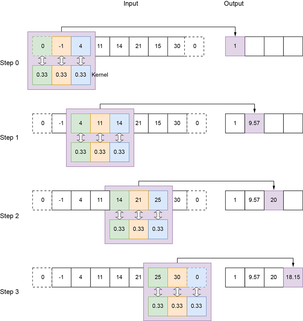
Figure 10.4 1D convolution with a local averaging kernel of size 3, stride 2, and zero padding
Let’s denote the input array’s domain by S. It’s a 1D grid:
S = [0, W − 1]
Every point in S is associated with a value Xx. Together, these values form the input X. On this grid of input points, we define a subgrid So of output points. So is obtained from S by applying stride-based stepping on the input. Assuming s = [sW] denotes the stride, the first slide stop has the top-left corner of the rope at (x = 0). The next slide stop is at (x = sW), and the next is (x = 2sW), and so on. When we reach the right end, we stop. Overall, the output grid consists of the slide-stop points at which the top-left corner of the kernel (ruler) rests as it sweeps over the input volume: that is, So = {(x = 0), (x = sW)⋯,}. There is an output for each point in So.
Equation 10.1 shows how a single output value is generated in 1D convolution. X denotes input, Y denotes output, and W denote kernel weights:
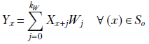
Equation 10.1
Note that when the kernel of dimension kW (ruler) has its origin on x, it covers all input pixels in the domain [x..(x + kW)]. These are the pixels participating in equation 10.1. Each of these input pixels is multiplied by the kernel element covering it. Match equation 10.1 with figures 10.1, 10.2, and 10.3.
10.1.1 Curve smoothing via 1D convolution
In this section, we look at how to perform local averaging via convolution, from a physical and algebraic viewpoint, to get a comprehensive understanding. The 1D kernel with weight vector ![]() (shown in figure 10.1) essentially takes the moving average of successive sets of three input values. As such, it is a local averaging (aka smoothing) operator. This becomes apparent if we examine the plots of the raw input vector with regard to the input vector convolved with the kernel (figure 10.5). The input (solid line) weaves up and down, while the output is a smooth curve (dashed line) through the mean position of the input. In general, the output produced by convolving by a kernel with all equal weights (the weights must be normalized, meaning the sum of the weights is 1) is a smoothed (locally averaged) version of the input. Why do we want to smooth an input vector? Because it captures the broad trend in the input data while eliminating short-term fluctuations (often caused by noise). If you are familiar with Fourier transforms and frequency domains, you can see that this is essentially a low-pass filter, eliminating short-term, high-frequency noise and capturing the longer-term, low-frequency variation in the input data array.
(shown in figure 10.1) essentially takes the moving average of successive sets of three input values. As such, it is a local averaging (aka smoothing) operator. This becomes apparent if we examine the plots of the raw input vector with regard to the input vector convolved with the kernel (figure 10.5). The input (solid line) weaves up and down, while the output is a smooth curve (dashed line) through the mean position of the input. In general, the output produced by convolving by a kernel with all equal weights (the weights must be normalized, meaning the sum of the weights is 1) is a smoothed (locally averaged) version of the input. Why do we want to smooth an input vector? Because it captures the broad trend in the input data while eliminating short-term fluctuations (often caused by noise). If you are familiar with Fourier transforms and frequency domains, you can see that this is essentially a low-pass filter, eliminating short-term, high-frequency noise and capturing the longer-term, low-frequency variation in the input data array.
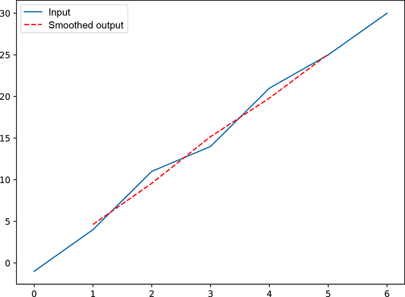
Figure 10.5 Graph of the input array solid) and output array (dashed) from figure 10.1. Note that the averaged) version of the input. Such local soothing captures the low-frequency (long-term) broad trend of the function by eliminating high-frequency (short-term) noise.
10.1.2 Curve edge detection via 1D convolution
As mentioned earlier, a convolution’s physical effect on an input array radically changes with the weights of the convolution kernel. Now let’s examine a very different kernel that detects edges in the input data.
An edge is defined as a sharp change in the values in an input array. For instance, if two successive elements in the input array have a large absolute difference in values, that is an edge. If we graph the input array (that is, plot the input array values in the y axis against the array indices), an edge will appear in the graph. For instance, consider the input array in figure 10.3 (graphed in figure 10.6). At indices 0 to 3, we have values in the neighborhood of 10. At index 4, the value jumps to 51. We say there is an edge between indices 3 and 4. The values then remain in the neighborhood of 50 at indices 4 to 7. Then they jump back to the neighborhood of 10 in the remaining indices. We say there is another edge between indices 7 and 8. The convolution we examine here will emit a high response (output value) exactly at the indices of the jump—3 and 7—while emitting a low response at other indices. This is an edge-detection convolution (filter). Why do we want to detect edges? Because edges are important for understanding images. Locations at which the signal changes rapidly provide more semantic clues than flat uniform regions. Experiments on the human visual cortex have established that humans pay more attention to locations where color or shade changes rapidly than to flat regions.
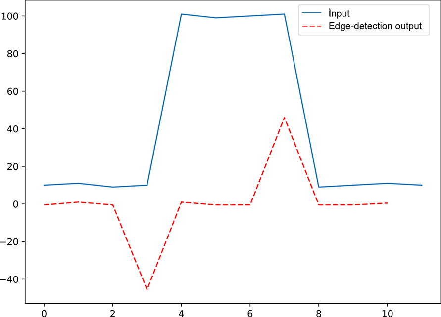
Figure 10.6 Graph of the input array solid) and output array (dashed) from figure 10.3. The output the input. Edges provide vital clues for understanding the signal.
10.1.3 One-dimensional convolution as matrix multiplication
Algebraically, the convolution with a kernel of size 3, stride 1, and valid padding can be shown as follows. Let the input array be
![]() = [x0 x1 x2 x3 x4 … xn–3 xn–2 xn-1]
= [x0 x1 x2 x3 x4 … xn–3 xn–2 xn-1]
The convolving kernel is a matrix of weights of size 3; let’s denote it as
![]() = [w0 w1 w2]
= [w0 w1 w2]
As shown in figure 10.1, in step 0 of the convolution, we place this kernel on the 0th element of the input x0. Thus, w0 falls on x0, w1 falls on x1, and w2 falls on x2:
[x0 x1 x2 x3 x4 … xn–3 xn–2 xn-1],
where the bold typeface identifies the input elements aligned with kernel weights. We multiply elements on corresponding positions and sum them, yielding the 0th element of the output y0 = w0x0 + w1x1 + w2x2. Then we shift the kernel by one position (assuming the stride is 1; if the stride were 2, we would move the kernel two positions, and so on). So w0 falls on x1, w1 falls on x2, and w2 falls on x3:
[x0 x1 x2 x3 x4 … xn–3 xn–2 xn-1]
Again, we multiply elements at corresponding positions and sum them, yielding the first element of the output y1 = w0x1 + w1x2 + w2x2. Similarly, in the next step, we right-shift the kernel one more time:
[x0 x1 x2 x3 x4 … xn]
The corresponding output is y2 = w0x2 + w1x3 + w2x4. Overall, a stride 1, valid padding convolution of a vector ![]() with a weight kernel
with a weight kernel ![]() yields the output
yields the output
Can you see what is happening? We are effectively taking linear combinations (see section 2.9) of successive sets of kernel_size here, 3) input elements. In other words, the output is a moving weighted local sum of the input array elements. Depending on the actual weights, we are extracting local properties of the input.
For valid padding, the last output is yielded by
[x0 x1 x2 x3 x4 … xn–3 xn–2 xn-1]
which generates the output
yn − 3 = w0xn − 3 + w1xn − 2 + w2xn − 1
For the same zero padding, the last output is yielded by
[x0 x1 x2 x3 x4 … xn-1 0 0]
which generates the output
yn−1 = w0 ⋅ xn−1 + w1 ⋅ 0 + w2 ⋅ 0
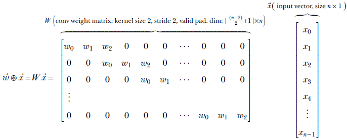
In section 8.3.1, we saw that the FC (aka linear) layer can be expressed as a multiplication of the input vector by a weight matrix. Now, we will express convolution as matrix-vector multiplication. The weight matrix has a block-diagonal structure, as shown in equation 10.2. It is a special case of equation 8.8. As such, the forward propagation equation 8.7 and backpropagation equations 8.31 and 8.33 are still applicable. Thus, forward propagation and backpropagation training) through convolution proceeds exactly as with FC layers.
Equation 10.2 expresses kernel_size 3, stride 1, valid padding convolution as a multiplication of a weight matrix W with input vector ![]() :
:
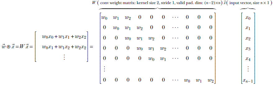
Equation 10.2
Notice the sparse, block-diagonal nature of the weight matrix in equation 10.2. This is characteristic of convolution weight matrices. Each row contains all the kernel weights at contiguous positions. The size of the kernel is typically much less than the input vector size. Of course, for matrix multiplication to be possible, the number of columns in the weight matrix must match the size of the input vector. Thus, there are many vacant positions in the row besides those occupied by kernel weights. We fill these vacant elements with zeros. Each row of the weight matrix thus has all the kernel weights appearing somewhere contiguously, and the rest of the row is filled with zeros. The position of kernel weights shifts rightward with each successive row. This is what gives the block-diagonal appearance to the weight matrix. It also simulates the sliding of the kernel required for convolution. Each row represents a specific slide stop and generates one element of the output vector. Since the kernel is at a fixed position of the row and all other row elements are zero, only the input elements corresponding to the kernel positions are picked up. Other input elements are multiplied by zero: that is, they are ignored.
Equation 10.2 depicts a stride of 1. For instance, if the stride is 2, the kernel weights will shift by two positions in successive rows. This is shown in equation 10.3:
Equation 10.3
Note that while equation 10.3 provides a conceptual matrix-multiplication view of convolution, it is not the most efficient way of implementing convolution. PyTorch and other deep learning software have extremely efficient ways of implementing convolution.
10.1.4 PyTorch- One-dimensional convolution with custom weights
We have discussed the convolution of a 1D input vector with two specific 1D kernels. We have seen that a kernel with uniform weights, such as ![]() , results in local smoothing of the input vector, whereas a kernel with antisymmetric weights, such as
, results in local smoothing of the input vector, whereas a kernel with antisymmetric weights, such as ![]() , results in an output vector that spikes at the edge locations in the input vector. Now we will see how to set the weights of a 1D kernel and perform 1D convolution with that kernel in PyTorch.
, results in an output vector that spikes at the edge locations in the input vector. Now we will see how to set the weights of a 1D kernel and perform 1D convolution with that kernel in PyTorch.
NOTE This is not a typical PyTorch operation. The more typical operation is to create a neural network with a convolution layer (where we specify the size, stride, and padding but not the weights) and then train the network so that the weights are learned. We usually don’t care about the exact values of the learned weight. Then why are we discussing how to set the weights of a kernel in PyTorch? Mainly to show how convolution works in PyTorch, the various parameters of the convolution object, and so forth.
Listing 10.1 PyTorch code for 1D local averaging convolution
import torch

x = torch.tensor(                                          ①
        [-1.,  4., 11., 14., 21., 25., 30.])

w = torch.tensor([0.33, 0.33, 0.33])                       ②

x = x.unsqueeze(0).unsqueeze(0)
w = w.unsqueeze(0).unsqueeze(0)                            ③

conv1d = torch.nn.Conv1d(1, 1, kernel_size=3,              ④
            stride=1, padding=[0], bias=False)

conv1d.weight = torch.nn.Parameter(w, requires_grad=False) ⑤

with torch.no_grad():                                      ⑥

    y = conv1d(x)                                          ⑦
① Instantiates a noisy input vector. Follows equation y = 5x
② Instantiates the weights of the convolutional kernel
③ PyTorch expects inputs and weights to be of the form N × C × L, where N is the batch size, C is the number of channels, and L is the sequence length. Here, N and C are 1. torch.unsqueeze converts our L-length vector into a 1 × 1 × L tensor.
④ Instantiates the smoothing kernel
⑤ Sets the kernel weights
⑥ Instructs PyTorch to not compute gradients since we currently don’t require them
⑦ Runs the convolution
Listing 10.2 PyTorch code for 1D edge detection
import torch

x = torch.tensor(                                           ①
        [10.,  11., 9., 10., 101., 99.,
         100., 101., 9., 10., 11., 10.])

w = torch.tensor([0.5, -0.5])                               ②

x = x.unsqueeze(0).unsqueeze(0)                             ③
w = w.unsqueeze(0).unsqueeze(0)

conv1d = torch.nn.Conv1d(1, 1, kernel_size=3,               ④
            stride=1, padding=[0], bias=False)

conv1d.weight = torch.nn.Parameter(w, requires_grad=False)  ⑤


with torch.no_grad():                                       ⑥

    y = conv1d(x)                                           ⑦
① Instantiates the input vector with edges
② Instantiates the weights of the edge-detection kernel
③ Converts the inputs and weights to 1 × 1× L
④ Instantiates the edge-detection kernel
⑤ Sets the kernel weights
⑥ Instructs PyTorch to not compute gradients since we currently don’t require them
⑦ Runs the convolution
These listings show how to perform 1D convolution in PyTorch using the torch.nn. Conv1d class. This is typically used in larger neural networks like those in subsequent chapters. We can alternatively use torch.nn.functional.conv1d to directly invoke the mathematical convolution operation. This takes input and weight tensors and returns the convolved output tensor, as shown in listing 10.3.
Listing 10.3 PyTorch code directly invoking the convolution function
import torch

x = torch.tensor(                              ①
        [10.,  11., 9., 10., 101., 99.,
         100., 101., 9., 10., 11., 10.])

w = torch.tensor([0.5, -0.5])                  ②

x = x.unsqueeze(0).unsqueeze(0)                ③
w = w.unsqueeze(0).unsqueeze(0)

y = torch.nn.functional.conv1d(x, w, stride=1) ④
① Instantiates the input tensor
② Instantiates the weight tensor
③ Converts the inputs and weights to 1 × 1 × L
④ Runs the convolution
10.2 Convolution output size
Consider a kernel of size k sliding over an input of size n with stride s. Given a kernel of size k, if the left end is at index l, the right end is at index l + (k − 1). Each shift advances the left (as well as the right) end of the kernel by s. If the initial position of the kernel was at index 0, then after m shifts, the left end is at ms. Correspondingly, the right end is at ms + (k − 1). Assuming valid padding, this right-end position must be less than or equal to (n − 1) (the last valid position of the input array).
How many times can we shift before the kernel spills out of the input? In other words, what is the maximum possible value of m, such that
ms + (k − 1) ≤ (n − 1)
The answer is
![]()
But each shift produces one output value. The output size of the convolution, o, with valid padding, is m + 1 (the plus one is to account for the initial position). Hence,
![]()
If we are zero-padding with p zeroes on each side of the input, the input size becomes n + 2p. The corresponding output size is
![]()
Equation 10.4
This can be extended to an arbitrary number of dimensions by repeating it for each dimension.
10.3 Two-dimensional convolution: Graphical and algebraic view
It is often said that an image is worth a thousand words. What is an image? As far as deep learning is concerned, it is a discrete two-dimensional entity—a 2D array of pixel values describing a scene at a fixed time. Each pixel represents a color intensity value. The color value can be a single element representing a gray level, or it can be three-dimensional, corresponding to R(ed), G(reen), B(lue) intensity values. (You may want to revisit section 2.3 before proceeding.)
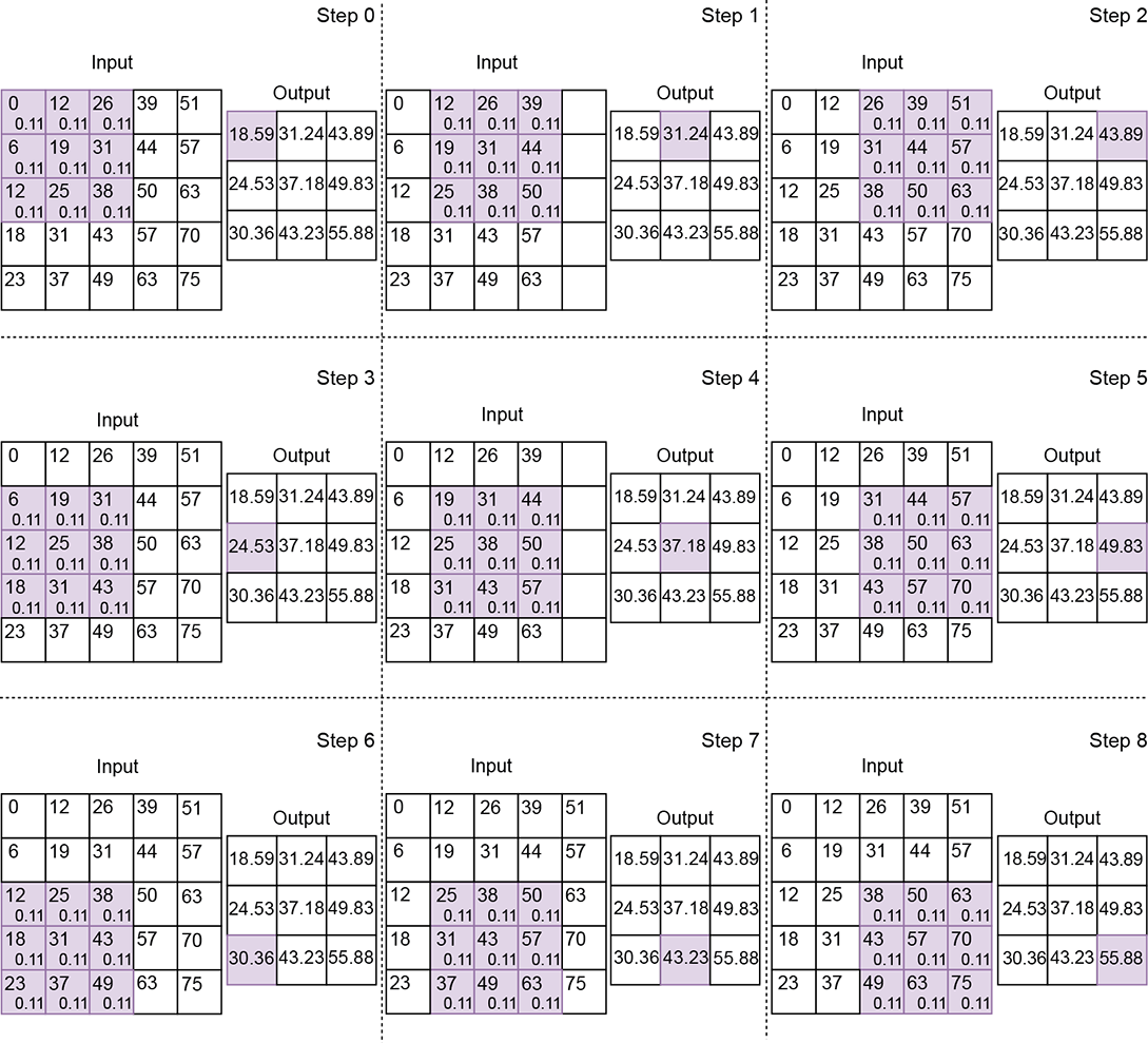
Figure 10.7 2D convolution with a local averaging kernel of size [3,3], stride [1,1], and valid padding. Each pixel is shown as a small rectangle, with the pixel’s gray level written in the rectangle. The shaded order. Successive steps indicate slide stops. For each pixel that is overlapped by the kernel, the weight of the kernel element falling on it is written in small font.
At the time of this writing, image analysis is the most popular application of convolution. These applications use convolution to extract local patterns. How do we do this? In particular, can we rasterize the image (thus converting it into a vector) and use one-dimensional convolution?
The answer is no. To see why, examine figure 10.7. What is the spatial neighborhood of the pixel at location (x = 0, y = 0)? If we define the neighborhood of a pixel as the set of pixels within a Manhattan distance of [2,2] with that pixel at the top-left corner, the neighborhood of (x = 0, y = 0) consists of the set of pixels covered by the shaded rectangle in figure 10.7, step 0. But these pixels will not be neighboring elements in a rasterized array representation of the image. For instance, the pixel (x = 0, y =1), with value 6, is the fifth element in the rasterized array and, as such, will not be considered a neighbor of (x = 0, y = 0), which is the 0th element in the rasterized array. Two-dimensional neighborhoods are not preserved by rasterization. So, two-dimensional convolution has to be a specialized operation beyond merely rasterizing 2D arrays into 1D and applying 1D convolution.
The best way to visualize 2D convolution is to imagine a wall (the input image) over which a tile the kernel) is sliding:
-
In figures 10.7, 10.8 and 10.9, the shaded rectangle depicts the tile (kernel), while the larger white rectangle containing it depicts the wall (input image). Successive steps in the figure represent successive positions (aka slide stops) of the sliding tile. Notice that the shaded rectangle occupies a different position in each step.
-
Tiles in successive positions during sliding can overlap. They overlap by varying amounts in figures 10.7, 10.8, and 10.9.
-
The wall and the tile are discrete 2D arrays in reality. At each slide stop, the tile array elements rest on a subset of wall array elements.
-
We multiply each input array element by the kernel element resting on it and sum the products. This is equivalent to taking a weighted sum of the input (wall) elements that fall under the current position of the kernel (tile), with the kernel elements serving as weights. This weighted sum is emitted as a single output element. One output element results from each slide stop of the tile. As the tile slides over the entire wall, left to right and top to bottom, a 2D output array is generated.
In 2D convolution, the input array, kernel size, and stride are all 2D vectors. Just as in 1D convolution, the following entities are defined for 2D convolution:
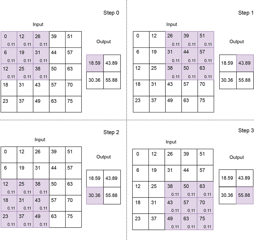
Figure 10.8 2D convolution with a local averaging kernel of size [3,3], stride [2,2], and valid padding
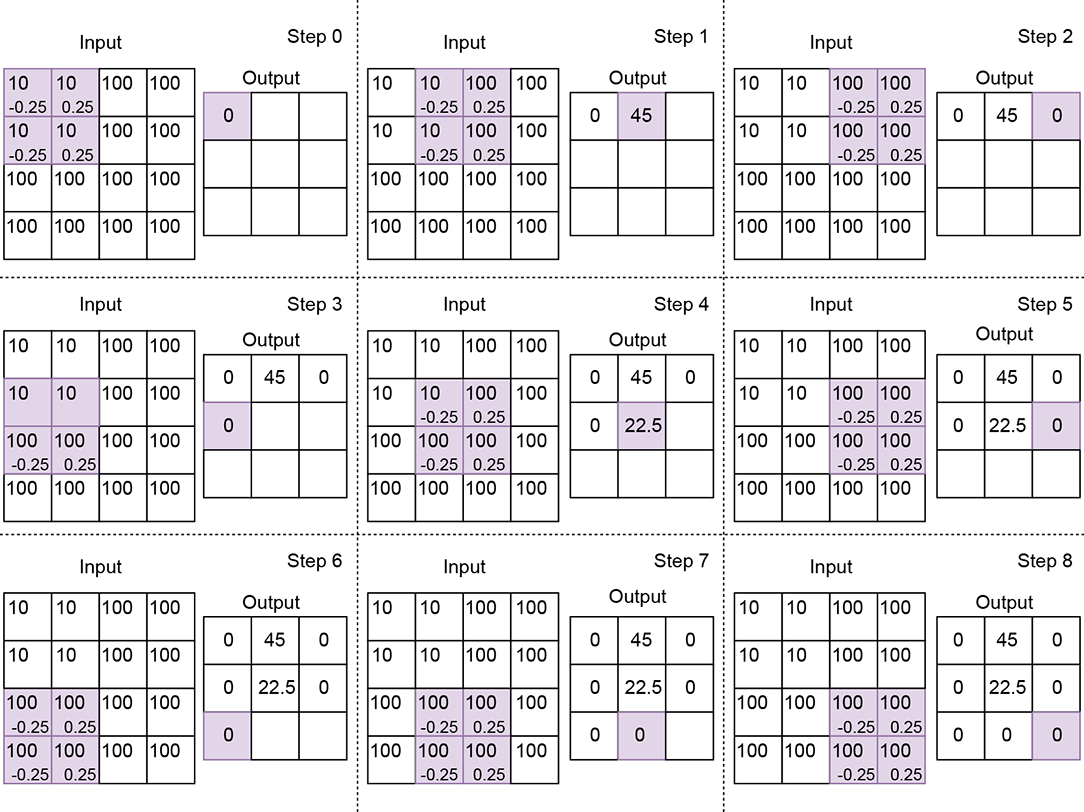
Figure 10.9 2D convolution with an edge-detection kernel of size 2, stride 1, and valid padding. Not all slide stops that is, steps) are shown. Notice how the output is zero at a uniform location but spikes when one-half of the kernel falls on low values while the other half falls on high values.
-
Input—A two-dimensional array. We typically use the symbol [H, W] indicating the height and width of the array, respectively) to represent the input array size in 2D convolution. In figure 10.7, H = 5, W = 5.
-
Output—A two-dimensional array. We typically use the symbol
 = [oH, oW] to represent output array dimensions in 2D convolution. For instance, in figure 10.7, = [3,3]. In section 10.2, we saw how to compute the output size for a single dimension. We have to repeat that computation once per dimension to obtain the output size in higher dimensions.
 -
Kernel—A small two-dimensional array of weights whose size is a parameter of the convolution. We typically use the symbol
 = [kH, kW] to represent the kernel size (height, width) in 2D convolution. If (x, y) denotes the current position of the top-left corner of the 2D kernel, the bottom-right corner is at (x + kW − 1, y + kH − 1). In figure 10.7, = [3,3]; in figure 10.9, = [2,2].
 -
Stride—The number of input elements over which the kernel slides on completing a single step. We typically use the symbol
 = [sH, sW] to represent the stride size (height, width) in 2D convolution. If (x, y) denotes the current position of the top-left corner of the 2D kernel, the next shift will put the top-left corner of the kernel at (x + sW, y) see, for instance, the transition from step 0 to step 1 or step 1 to step 2 in figure 10.7). If this transition causes portions of the tile to fall outside the wall—that is, x + sW ≥ W—we set the next slide position such that the top-left corner of the kernel falls on (0, y + 1) (see, for instance, the transition from step 2 to step 3 or step 5 to step 6 in figure 10.7). If y + sH ≥ H, we stop sliding. Stride size is a parameter of the convolution. In figure 10.7, = [1,1]; in figure 10.8, stride is = [2,2]. As in the 1D case, a stride of = [1,1] means there is a slide stop at each successive element of the input. So, the output has roughly the same number of elements as the input (they may not be exactly equal because of padding). A stride of = [2,2] means each row of the input will yield half the row size worth of output elements, and each column will generate half the column size worth of output elements. Hence, the output size is roughly a quarter of the input size. Overall, the reduction factor of the input-to-output size roughly matches the product of the elements in the stride vector.
 -
Padding—As the kernel slides toward the extremity of the input array along the width and/or height, parts of it may fall outside the input array. In other words, part of the kernel falls over ghost input elements. As in the 1D case, we deal with this via padding. Padding strategies in 2D convolution are straightforward extensions from 1D:
-
Valid padding—We stop sliding whenever any element of the kernel falls outside the input array, either in width and/or in height. No ghost input elements are involved; the entire kernel always falls on valid input elements (hence the name valid).
-
Same (zero) padding—Here, we do not want to stop early. We keep sliding as long as the top-left corner of the kernel falls on a valid input position. So, if the stride is 1, 1, the output size will match the input size (hence the name same). When we slide near the end of an input row (right extremity of the input), the right-most columns of the kernel will fall outside the input. Similarly, when we slide toward the bottom of the input, the bottom rows of the kernel will fall outside. If we slide near the bottom-right corner of the input, both the right-most columns and bottommost rows will fall outside the input. The rule is that all ghost input values outside the true boundaries of the input array are replaced by zeros.
-
Let’s denote the input image domain by S. It is a 2D grid whose domain is
S = [0, H − 1] × [0, W − 1]
Every point in S is a pixel with a color value (which can be a scalar—a gray-level value—or a vector of three values, R, G, B. On this grid of input points, we define a subgrid So of output points. So is obtained from S by applying stride-based stepping on the input. Assuming ![]() = [sH, sW] denotes the 2D stride vector, the first slide stop has the top-left corner of the brick at
= [sH, sW] denotes the 2D stride vector, the first slide stop has the top-left corner of the brick at ![]() 0 ≡ (y = 0, x = 0). The next slide stop is at
0 ≡ (y = 0, x = 0). The next slide stop is at ![]() 1 ≡ (y = 0, x = sW), and the next is at
1 ≡ (y = 0, x = sW), and the next is at ![]() 2 ≡ (y = 0, x = 2sW). When we reach the right end, we increment y. Overall, the output grid consists of the slide-stop points where the top-left corner of the kernel (brick) rests as it sweeps over the input volume: So = {
2 ≡ (y = 0, x = 2sW). When we reach the right end, we increment y. Overall, the output grid consists of the slide-stop points where the top-left corner of the kernel (brick) rests as it sweeps over the input volume: So = {![]() 0,
0, ![]() 1, … }. There is an output for each point in So.
1, … }. There is an output for each point in So.
The kernel also has two dimensions (in practice, it has two more dimensions corresponding to the input channels and batch—we are ignoring them now for simplicity—as discussed in section 10.3.3). Equation 10.5 shows how a single output value is generated in 2D convolution. X denotes input, Y denotes output, and W denote kernel weights:
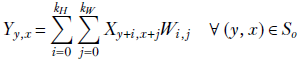
Equation 10.5
Note that the kernel (tile) has its origin on Xy, x. Its dimensions are (kH, kW). So, it covers all input pixels in the domain [y..(y + kH)] × [x..(x + kW)]. These are the pixels participating in equation 10.5. Each of these input pixels is multiplied by the kernel element covering it. Match equation 10.5 with figures 10.7, 10.8, and 10.9.
10.3.1 Image smoothing via 2D convolution
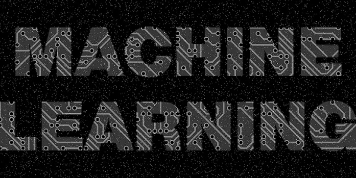
In section 10.1.1, we discussed one-dimensional local smoothing. We observed how it gets rid of local fluctuations so that longer-term patterns are discernible more cleanly. The same thing happens in two dimensions. Figure 10.10 shows an image with some text written on a background with salt-and-pepper noise. The noise has no semantic significance; it is the text that needs to be analyzed (perhaps via optical character recognition). We can eliminate the noise via 2D convolution using a kernel with uniform weights, such as
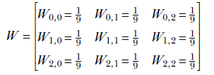
The resulting denoised/smooth image is shown in figure 10.11. What does the uniform kernel do? To see that, look at figure 10.8. It should be obvious that the kernel causes each output pixel to be a weighted local average of the neighboring 3 × 3 input pixels.
(a) Input image

(b) Smoothed/denoised output image
Figure 10.10 Denoising/smoothing a noisy image by applying 2D convolution 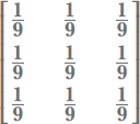 to figure 10.11a
NOTE Fully functional code for image smoothing, executable via Jupyter Notebook, can be found at http://mng.bz/aDM7.
10.3.2 Image edge detection via 2D convolution
Not all pixels in an image have equal semantic importance. Imagine a photograph of a person standing in front of a white wall. The pixels belonging to the wall are uniform in color and uninteresting. The pixels that yield the most semantic clues are those belonging to the silhouette: the edge pixels. This agrees with the science of human vision, where, as we mentioned earlier, experiments indicate that the human brain pays more attention to regions with sharp changes in color. Humans treat sound in a very similar fashion, ignoring uniform buzz such sounds often induce sleep) but becoming alert when the volume or frequency of the sound changes. Thus, identifying edges in an image is vital for image understanding.
Edges are local phenomena. As such, they can be identified by 2D convolution with specially chosen kernels. For instance, the vertical edges in figure 10.11b were produced by performing 2D convolution on the image in figure 10.11a using the kernel
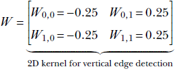
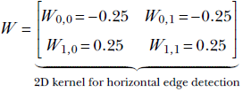
Likewise, the vertical edges in figure 10.11c were produced by performing 2D convolution on the image in figure 10.11a using the kernel
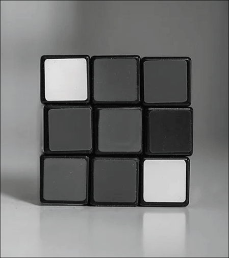
(a) Input image
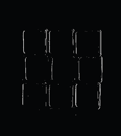
(b) Vertical edges detected by applying 2D convolution ![]() to figure 10.11a
to figure 10.11a
(c) Horizontal edges detected by applying 2D convolution ![]() to figure 10.11a
to figure 10.11a
Figure 10.11 image often helps us analyze the image.
How do these kernels identify edges? To see this, look at figure 10.9. In a neighborhood with equal pixel values (for example, a flat wall), the kernel in figure 10.11b will yield zero (the positive and negative kernel elements fall on equal values, and their weighted sum is zero). Thus this kernel suppresses uniform regions. On the other hand, it has a high response if there is a sharp jump in color (the negative and positive halves of the kernel fall on very different values, and the weighted sum is a large negative or large positive).
NOTE Fully functional code for edge detection, executable via Jupyter Notebook, can be found at http://mng.bz/g4JV.
10.3.3 PyTorch- 2D convolution with custom weights
We have discussed the convolution of 2D input arrays with two specific 2D kernels. We have seen that a kernel with uniform weights, such as  , results in local smoothing of the input array, whereas a kernel with antisymmetric weights, such as
  , results in an output array that spikes at the edge locations in the input array. Now we will see how to set the weights of a 2D kernel and perform 2D convolution with that kernel in PyTorch.
NOTE This is not a typical PyTorch operation. The more typical operation is to create a neural network with a convolution layer (where we specify the size, stride, and padding but not the weights) and then train the network so that the weights are learned. We usually don’t care about the exact values of the learned weight. A sample neural network with a 2D convolution layer can be seen in section 10.6.
Listing 10.4 shows local averaging convolution in two dimensions. While we saw in section that input arrays are 2D tensors of shape H × W, the PyTorch interface to convolution expects 4D tensors of shape N × C × H × W as input:
-
The first dimension, N, stands for the batch size. In a real neural network, inputs are fed in minibatches instead of one input instance at a time (this is for efficiency reasons, as discussed in section 9.2.2). N stands for the number of input images contained in the minibatch.
-
The second dimension, C, stands for the number of channels. For the input to the entire neural network, in the case of RGB images, we have three channels R (red), G (green), and B (blue); in the case of grayscale images, we only have a single channel. For other layers, the number of channels can be anything, depending on the neural network’s architecture. Typically, layers further from the input and closer to the output have more channels. Only channels at the grand input have fixed, clearly discernible physical significance (like R, G, B). Channels at the input to successive layers do not.
-
The third dimension, H, stands for the height.
-
The fourth dimension, W, stands for the width.
The weight tensor of a PyTorch Conv2D object has to be a 4D tensor. The listing shows a single grayscale image of size 5 × 5 as input. Hence N = 1, C = 1, H = 5, and W = 5. x is instantiated as a 2D tensor of size 5 × 5. To convert it to a 4D tensor, we use the torch.unsqueeze() function, which adds an extra dimension to the input.
Listing 10.4 PyTorch code for 2D local averaging convolution
import torch

x = load_img()                                             ①

w = torch.tensor(                                          ②
    [
        [0.11, 0.11, 0.11],
        [0.11, 0.11, 0.11],
        [0.11, 0.11, 0.11]
    ]
)

x = x.unsqueeze(0).unsqueeze(0)                            ③
w = w.unsqueeze(0).unsqueeze(0)

conv2d = torch.nn.Conv2d(1, 1, kernel_size=2,
                    stride=1, bias=False)                  ④

conv2d.weight = torch.nn.Parameter(w, requires_grad=False) ⑤


with torch.no_grad():                                      ⑥


    y = conv2d(x)                                          ⑦
① Loads a noisy grayscale input image
② Instantiates the weights of the convolutional kernel
③ PyTorch expects inputs and weights to be of the form N × C × H × W, where N is the batch size, C is the number of channels, H is the height, and W is the width. Here, N = 1 because we have a single image. C = 1 because we are considering a grayscale image. H and W are both 5 because the input is a 5 × 5 array. unsqueeze converts our 5 × 5 tensor into a 1 × 1 × 5 × 5 tensor.
④ Instantiates the 2D smoothing kernel
⑤ Sets the kernel weights
⑥ Instructs PyTorch to not compute gradients since we currently don’t require them
⑦ Runs the convolution
Listing 10.5 PyTorch code for 2D edge detection
import torch

x = load_img()                                             ①

w = torch.tensor(                                          ②
        [[-0.25, 0.25],
        [-0.25, 0.25]]
    )

x = x.unsqueeze(0).unsqueeze(0)                            ③
w = w.unsqueeze(0).unsqueeze(0)

conv2d = torch.nn.Conv2d(1, 1, kernel_size=2,              ④
                    stride=1, bias=False)

conv2d.weight = torch.nn.Parameter(w, requires_grad=False) ⑤

with torch.no_grad():                                      ⑥

    y = conv2d(x)                                          ⑦
① Loads a grayscale input image with edges
② Instantiates the weights of the convolutional kernel
③ Converts the inputs to 1 × 1 × 4 × 4
④ Instantiates a 2D edge-detection kernel
⑤ Sets the kernel weights
⑥ Instructs PyTorch to not compute gradients since we currently don’t require them
⑦ Runs the convolution
10.3.4 Two-dimensional convolution as matrix multiplication
In section 10.1.3, we saw how 1D convolution can be viewed as multiplying the input vector by a block-diagonal matrix (shown in equation 10.3). The idea can be extended to higher dimensions, although the matrix of weights becomes significantly more complex. Nonetheless, it is important to have a mental picture of this matrix. Among other things, it will help us better understand transposed convolution. In this matrix multiplication-oriented view of 2D convolution, the input image is represented as a rasterized 1D vector. Thus, an input matrix of size m × n becomes an mn-sized vector. The corresponding weight matrix has rows of length mn. Each row corresponds to a specific slide stop.
For ease of understanding, let’s consider an input image with [H, W] = [4,4] (never mind that this image is unrealistically small). On this image, we are performing 2D convolution with a [kH, kW] = [2,2] kernel with stride [sH, sW] = [1,1]. The situation is exactly as shown in figure 10.9. The input image X with size H = 4, W = 4
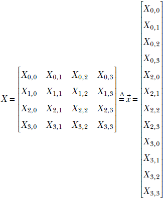
rasterizes to the input vector ![]() of length 4 * 4 = 16. Let the kernel weights be denoted as
of length 4 * 4 = 16. Let the kernel weights be denoted as ![]() Consider the successive slide stops (steps in figure 10.9). The exact elements of the rasterized input vector that are multiplied by kernel weights for a specific step are shown below—these correspond to the shaded items for the same steps in figure 10.9: 2D convolution between an image X and a kernel W, denoted Y = W ⊛ X, in the special case of an input image with [H, W] = [4,4]. For this image, 2D convolution with a [kH, kW] = [2,2] kernel with stride [sH, sW] = [1,1] and valid padding can be expressed as the following matrix multiplication:
Consider the successive slide stops (steps in figure 10.9). The exact elements of the rasterized input vector that are multiplied by kernel weights for a specific step are shown below—these correspond to the shaded items for the same steps in figure 10.9: 2D convolution between an image X and a kernel W, denoted Y = W ⊛ X, in the special case of an input image with [H, W] = [4,4]. For this image, 2D convolution with a [kH, kW] = [2,2] kernel with stride [sH, sW] = [1,1] and valid padding can be expressed as the following matrix multiplication:
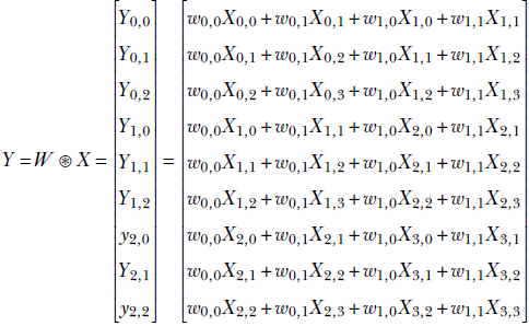
This can be expressed as
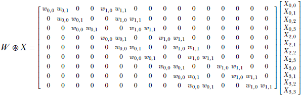
Equation 10.6
Note the following:
-
The 2D convolution weight matrix shown in equation 10.6 is for the special case, but it illustrates the general principle.
-
The 2D convolution weight matrix is block diagonal, just like the 1D version. The kernel weights are placed precisely to emulate figure 10.9.
-
The convolution weight matrix has 9 rows and 16 columns. Thus it takes a input vector rasterized from a 4 × 4 input image) and generates a output matrix (which can be folded into a 3 × 3 convolution output image.
10.4 Three-dimensional convolution
If a picture is worth a thousand words, a video is worth 10,000 words. Videos are a rich source of information about dynamic real-life scenes. As deep learning-based image analysis (2D convolution) is becoming more and more successful, at the time of this writing, video analysis is becoming the next research frontier to conquer.
Videos are essentially three-dimensional entities. The representation is discrete in all three dimensions. The three dimensions correspond to space, which is two-dimensional, having height and width, and time. A video consists of a sequence of frames. Each frame is an image: a discrete 2D array of pixels. A frame represents the entire video scene at a specific (sampled) point. A pixel in a frame represents the color of a sampled location in space belonging to the scene at the time corresponding to the frame. Thus a video is a sequence of frames representing the dynamic scene at a sampled set of discrete points (pixels) in space and time. The video extends over a spatio-temporal volume (aka ST volume), which can be imagined as a cuboid. Each cross-section is a rectangle representing a frame. This is shown in figure 10.12.
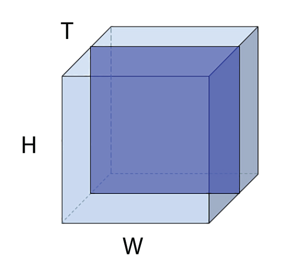
Figure 10.12 A spatio-temporal volume light-shaded cuboid) representing a video. Individual frames of the video are cross-sectional rectangles in this ST volume. A single frame is also shown in darker shading.
To analyze the video, we need to extract local patterns from this 3D volume. Can we do it via repeated 2D convolutions?
The answer is no. There is extra information when we view the successive frames together, which is absent when we view the frames one at a time. For instance, imagine you are presented with an image of a half-open door. From that single image, can you determine whether the door is opening or closing? No, you cannot. To make that determination, we need to see several successive frames. In other words, analyzing a video one frame at a time robs us of a vital modality of information: motion, which can be understood only if we analyze multiple successive frames together. This is why we need 3D convolution.
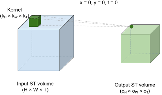
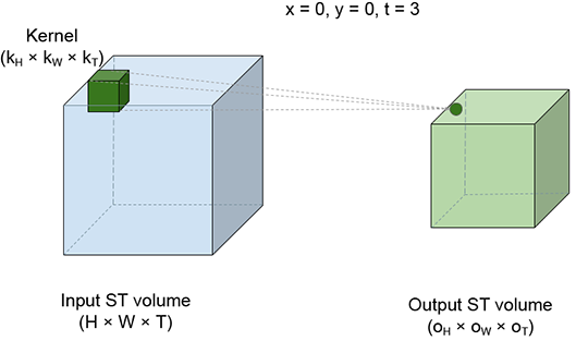
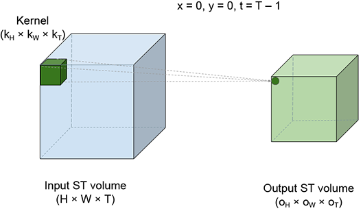
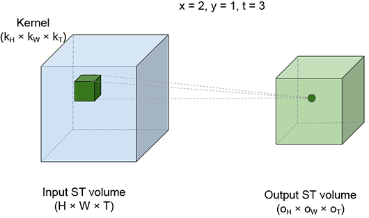
The best way to visualize a 3D convolution is to imagine a brick sliding over the entire volume of a room. The room corresponds to the ST volume of the video input to the convolution. The brick corresponds to the kernel. While sliding, the brick stops at successive positions; we call these slide stops. Figure 10.13 shows four slide stops at different positions. Each slide stop emits one output point. As the brick sweeps over the entire input ST volume, an output ST volume is generated. At each slide stop, we multiply each input pixel value by the kernel element covering it and take a sum of the products. This is effectively a weighted sum of all the input (room) elements covered by the kernel (brick), with the covering kernel elements serving as the weights.
(a) slide stop x = 0, y = 0, t = 0.
(b) slide stop x = 0, y = 0, t = 0.
(c) slide stop x = 0, y = 0, t = 0.
(d) slide stop x = 0, y = 0, t = 0.
Figure 10.13 Spatio-temporal view of 3D convolution. The larger, light-shaded cuboid on the left of each figure represents the input ST volume (room). The small, dark-shaded cuboid inside the room represents the kernel brick). The brick slides all over the room’s internal volume. Neighboring positions of the brick may overlap in volume. Each position of the brick represents a slide stop; a weighted sum is taken of all points in the room (input points) covered by the brick. The brick point kernel value) covering each input point serves as the weight. Four different slide stops are shown. Each slide stop generates a single output point. As the brick sweeps the input volume, an output ST volume the smaller light-shaded cuboid) is generated.
Let’s denote the input ST volume by S. It is a 3D grid whose domain is
S = [0, T − 1] × [0, H − 1] × [0, W − 1]
Every point in S is a pixel with a color value (which can be a scalar—a gray-level value—or a vector of three values, R, G, B. On this grid of input points, we define a subgrid So of output points. So is obtained from S by applying stride-based stepping on the input. Assuming ![]() = [sT, sK, sW] denotes the 3D stride vector, the first slide stop has the top-left corner of the brick at
= [sT, sK, sW] denotes the 3D stride vector, the first slide stop has the top-left corner of the brick at ![]() 0 ≡ (t = 0, y = 0, x = 0). The next slide stop is at
0 ≡ (t = 0, y = 0, x = 0). The next slide stop is at ![]() 1 ≡ (t = 0, y = 0, x = sW), and the next is at
1 ≡ (t = 0, y = 0, x = sW), and the next is at ![]() 2 ≡ (t = 0, y = 0, x = 2sW). When we reach the right end, we increment y. When we reach the bottom, we increment t. When we reach the end of the room, we stop. So = {
2 ≡ (t = 0, y = 0, x = 2sW). When we reach the right end, we increment y. When we reach the bottom, we increment t. When we reach the end of the room, we stop. So = {![]() 0,
0, ![]() 1 … } are the points at which the top-left corner of the kernel (brick) rests as it sweeps over the input volume. There is an output for each point in So. The kernel also has three dimensions (in practice, it has two more dimensions corresponding to the input channels and batch—we are ignoring them now for simplicity—as discussed in section 10.4.2.1).
1 … } are the points at which the top-left corner of the kernel (brick) rests as it sweeps over the input volume. There is an output for each point in So. The kernel also has three dimensions (in practice, it has two more dimensions corresponding to the input channels and batch—we are ignoring them now for simplicity—as discussed in section 10.4.2.1).
Equation 10.7 shows how a single output value is generated in 3D convolution. X denotes the input, Y denotes the output, and W denote the kernel weights:
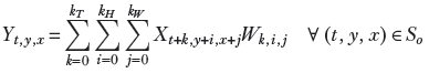
Equation 10.7
Note that the kernel (brick) has its origin on Xt, y, x. Its dimensions are (kT, kH, kW). So, it covers all input pixels in the domain [t..(t + kT)] × [y..(y + kH)] × [x..(x + kW)]. These are the pixels participating in equation 10.7. Each of these input pixels is multiplied by the kernel element covering it. Match equation 10.7 with figure 10.13.
10.4.1 Video motion detection via 3D convolution
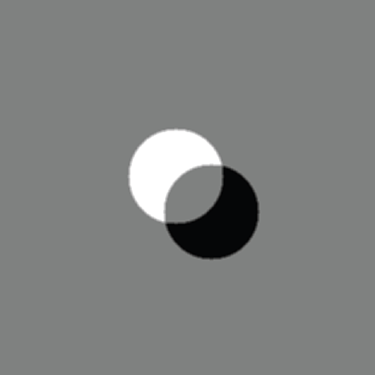
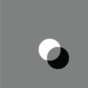
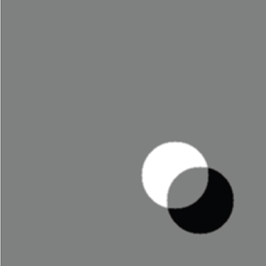
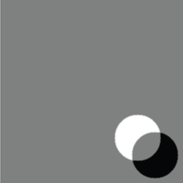
A moving object in a dynamic scene changes position from one video frame to another. Consequently, pixels are covered or uncovered at the boundary of motion. Pixels belonging to the background in one frame may be covered by the object in a subsequent frame and vice versa. If the background is a different color than the object, this will cause a color difference between pixels at identical spatial locations at different times, as illustrated in figure 10.14. The output of applying convolution to an ST volume is another ST volume. Figure 10.15 shows a few frames from the output resulting from applying our video motion detector to the input shown in figure 10.14.
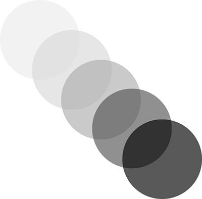
Figure 10.14 Successive frames of a synthetic video of a moving ball, shown in a superimposed fashion with gradually increasing opacity for illustration purposes
How does a kernel extract motion information from a set of successive frames? As mentioned earlier, motion causes pixels at the same position in successive frames to have different colors. However, a single isolated pair of pixels may have different colors due to noise—we cannot draw any conclusions from that. If we average the pixel values in a small neighborhood in one frame and average the pixel values in the same neighborhood in the subsequent frames, and these two averages are different, that is a more reliable way to estimate motion. Following is a 2 × 3 × 3 3D kernel to do exactly that—average pixel values in a 3 × 3 spatial neighborhood in two successive frames and subtract one from the other:
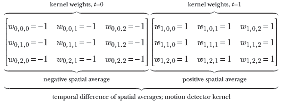
The result of the subtraction is high in regions of motion and low in regions of no motion. In this context, it is worthwhile to note that since the object is of uniform color, pixels within the object are indistinguishable. Consequently, no motion is observed at the center of the object; motion is observed only at the boundary. A few individual frames of the result of this 3D convolution are shown in figure 10.15.
NOTE Fully functional code for video motion detection, executable via Jupyter Notebook, can be found at http://mng.bz/enJQ.
(a) Output frame 0
(b) Output frame 1
(c) Output frame 2
(d) Output frame 3
Figure 10.15 Result of applying a 3D convolution motion detector to the synthetic video of a moving ball. Gray signifies “no motion"; most of the output frames are gray. White and black signify motion.
10.4.2 PyTorch- Three-dimensional convolution with custom weights
In section 10.4.1, we saw how to detect motion in a sequence of input images using 3D convolutions. In this section, we see how to implement this in PyTorch. The PyTorch interface to 3D convolutions expects 5-dimensional input tensors of the form N × C × D × H × W. In addition to the dimensions discussed in section 10.4, there is an additional dimension for the input channels. Thus, there is a separate brick for each input channel. We are combining (taking the weighted sum of) them all:
-
As discussed in the case of 2D convolutions (section 10.3.3), the first dimension N stands for the batch size minibatches are fed to a real neural network instead of individual input instances for efficiency reasons), and C stands for the number of input channels.
-
D stands for the sequence length. In our motion detector example, D represents the number of successive image frames fed to the 3D convolution layer.
-
The third dimension, H, stands for height, and the fourth dimension, W, stands for width.
In our motion detector example, we have a sequence of five grayscale images as input, each with height = 320 and width = 320. Since we are considering only a single image sequence, N = 1. All images are grayscale, which implies that C = 1. The sequence length, D, is equal to 5. H and W are both 320.
PyTorch expects the 3D kernels to be of the form Cout × Cin × kT × kH × kW:
-
The first dimension, Cout, represents the number of output channels. You can think of the convolutional kernel as a bank of 3D filters, where each filter produces one output channel. Cout is the number of 3D filters in the bank.
-
The second dimension, Cin, represents the number of input channels. This depends on the number of channels in the input tensor. When we are dealing with grayscale images, Cin is 1 at the grand input. For RGB images, Cin is 3 at the grand input. For layers further from the input, Cin equals the number of channels in the tensor fed to that layer.
-
The third, fourth, and fifth dimensions, kT, kH, and kW, represent the kernel sizes along the T, H, and W dimensions, respectively
In our motion detector example, we have a single kernel with kT=2, kH=3, and kW = 3. Since we only have a single kernel, Cout = 1. And since we are dealing with grayscale images, Cin is also 1.
Listing 10.6 PyTorch code for 3D convolution
import torch

images = load_images()                            ①

x = torch.tensor(images)                          ②

w_2d_smoothing = torch.tensor(                    ③
        [[0.11, 0.11, 0.11],
         [0.11, 0.11, 0.11],
         [0.11, 0.11, 0.11]]).unsqueeze(0)

w = torch.cat(
        [-w_2d_smoothing, w_2d_smoothing])        ④

x = x.unsqueeze(0).unsqueeze(0)                   ⑤

w = w.unsqueeze(0).unsqueeze(0)                   ⑥

conv3d = nn.Conv3d(1, 1, kernel_size=[2, 3, 3],   ⑦
                stride=1, padding=0, bias=False)
conv3d.weight = torch.nn.Parameter(w, requires_grad=False)

with torch.no_grad():                             ⑧

    y = conv3d(x)                                 ⑨
① Loads a sequence of five grayscale images with shape 320 × 320
② Converts to a tensor of shape T × H × W = 5 × 320 × 320
③ Instantiates a 2D smoothing kernel of shape 3 × 3. Pads an extra dimension so that two 2D kernels can be stacked together to form a 3D kernel.
④ Concatenates the 2D smoothing kernel and its inverted version along the first dimension to form a 3D kernel of shape 2 × 3 × 3
⑤ Converts the input tensor to N × C × T × H × W = 1 × 1 × 5 × 320 × 320
⑥ Converts the 3D kernel to Cout × Cin × kT × kH × kW = 1 × 1 × 2 × 3 × 3
⑦ Instantiates and sets the weights of the Conv3d layer
⑧ Instructs PyTorch to not compute gradients since we currently don’t require them
⑨ Runs the convolution
10.5 Transposed convolution or fractionally strided convolution
As usual, we examine this topic with an example. Consider a 1D convolution with kernel ![]() = [w0 w1 w2] of size 3, with valid padding. Let’s consider a special case where the input size n is 5. Following equation 10.2, this convolution can be expressed as a multiplication of a block-diagonal matrix W constructed from the weights vector
= [w0 w1 w2] of size 3, with valid padding. Let’s consider a special case where the input size n is 5. Following equation 10.2, this convolution can be expressed as a multiplication of a block-diagonal matrix W constructed from the weights vector ![]() , with input vector
, with input vector ![]() as follows:
as follows:
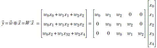
What happens if we multiply the output vector ![]() by the transposed matrix WT?
by the transposed matrix WT?
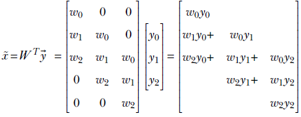
Following are some observations:
-
We haven’t quite recovered
 from
from  , but we have generated a vector, x̃, the same size as . Multiplying by the transpose of the weight matrix of the convolution performs a kind of upsampling, undoing the downsampling resulting from the forward convolution.
 -
It is impossible to recover
from . This is because when constructing from , we multiplied by W and converted a vector with five independent elements to a vector with three independent elements—some information was irretrievably lost. This intuition is consistent with the fact that a 5 × 3 matrix W is non-invertible: there is no W−1, so there is no way to get = W−1. -
During transpose convolution, we are distributing elements of
back to the elements of x̃ in the same proportion as when we were doing the forward convolution (see figure 10.16). This should remind you of backpropagation from chapter 8. There, in equation 8.24 right-hand side), we saw that for linear layers, forward propagation amounts to multiplying by an arbitrary weight matrix W (shown in equation 8.8). Backpropagation involves multiplying by the transpose of the same weight matrix (equation 8.31). The backpropagation does a proportional blame distribution—the loss is distributed back to the inputs in the same proportion as their contribution in creating the output. The same thing is happening here. Thus, multiplying by the transposed weight matrix in general distributes the output back in the same ratio in which it contributes to the output.
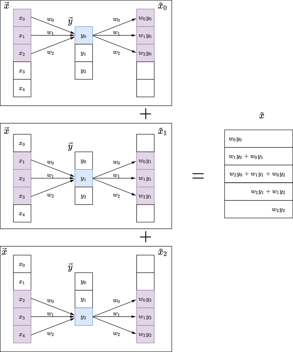
Figure 10.16 1D convolution and its transpose
The idea extends to higher dimensions. Figure 10.17 illustrates a 2D transpose convolution operation.
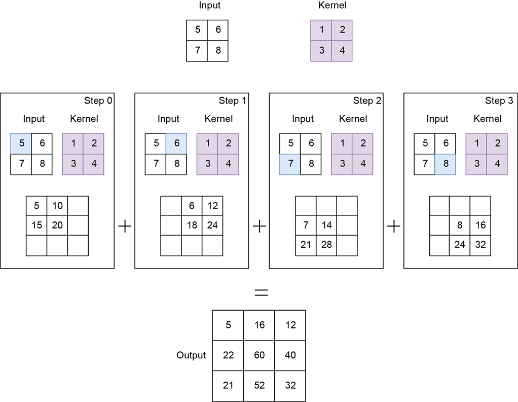
Figure 10.17 2D convolution and its transpose
10.5.1 Application of transposed convolution: Autoencoders and embeddings
Transposed convolution is typically required in autoencoders. We provide a very brief outline of autoencoders at this point to explain why they need transposed convolution. Most of the neural networks we have looked at so far are examples of supervised classifiers in that they take an input and directly output the class to which the input belongs. This is not the only paradigm possible. As hinted in section 6.9, we can also map an input to a vector often called the embedding, aka descriptor vector) that captures the essential aspects of the class of interest and throws away the variable aspects. For instance, if the class of interest is a human, then given an image, the embedding will only capture the features that recognize the humans in the image and ignore the background (sky, sea, forest, building, and so on).
The mapping from input to embedding is done by a neural network called an encoder. If the input is an image, the encoder typically contains a sequence of convolution layers.
How do we train this neural network? How do we define its loss? Well, one possibility is that the embedding must maintain fidelity to the original input: that is, we should be able to reconstruct (at least approximately) the input from the embedding. Remember, the embedding is smaller in size (with fewer degrees of freedom) than the input, so perfect reconstruction is impossible. Still, we can define loss as the difference (for example, Euclidean distance or binarized cross-entropy loss) between the original input and the reconstructed input.
How do we reconstruct the input from the embedding? This is where transposed convolution comes in. Remember, we did convolution (perhaps many times) in our encoder to generate the embedding. We can do a set of transposed convolutions on the embedding to generate a tensor of the same size as the input. The network to do this reconstruction is called the decoder. The decoder generates our reconstructed input.
We define a loss as the difference between the original and reconstructed input. We can train to minimize the loss and learn the weights of both the encoder and decoder. This is called end-to-end learning, and the encoder-decoder pair is called an autoencoder.
We train the autoencoder with many data instances, all belonging to the class of interest. Since it does not have the luxury of remembering the entire image (the embedding being smaller in size than the input), it is forced to learn how to retain the features common to all the training images: that is, the features that describe the class of interest. In our example, the autoencoder will learn to retain features that identify a human and drop the background. Note that this could also lead to a very effective compression technique—the embedding is a compact representation of the image in which only the objects of interest have been retained.
10.5.2 Transposed convolution output size
The output size of transposed convolution can be obtained by inverting equation 10.8:
o′ = (n′−1)s + k − 2p
Equation 10.8
For instance, transposed convolution with stride s = 1 on a ![]() of size n′ = 3 with valid padding p = 0) and a kernel of size k = 3 creates an output x̃ of size o′ = 5.
of size n′ = 3 with valid padding p = 0) and a kernel of size k = 3 creates an output x̃ of size o′ = 5.
10.5.3 Upsampling via transpose convolution
In the previous section, we briefly discussed autoencoders, where an encoder network maps an input image into an embedding and a decoder network tries to reconstruct the input image from the embedding. The encoder network converts a higher-resolution input into a lower-resolution embedding by passing the input through a series of convolution and pooling layers (we discuss pooling layers in detail in the next chapter). The decoder network, which tries to reconstruct the original image from the embedding, has to upscale/upsample a lower-resolution input into a higher-resolution output.
Many interpolation techniques, such as nearest neighbor, bilinear, and bicubic interpolation, can be used to perform this upsampling operation. These techniques typically use predefined mathematical functions to map lower-resolution inputs to higher-resolution outputs. However, a more optimal way to perform upsampling is through transpose convolutions, where the mapping function is learned during the training process instead of being predefined. The neural network will learn the best way to distribute the input elements across a higher-resolution output map so that the final reconstruction error is minimized (that is, the final output is as close to the original input image as possible). We do not get into the details of training an autoencoder in this chapter; however, we show how input images can be upsampled using transpose convolutions:
-
The input array is converted to a 4D tensor of shape N × Cin × H × W, where N is the batch size, Cin is the number of input channels, H is the height, and W is the width.
-
The kernel is a 4D tensor of shape Cin × Cout × kH × kW, where Cin is the number of input channels, Cout is the number of output channels, kH is the kernel height, and kW is the kernel width. Note how this differs from the regular 2D convolutional kernel, which is expected to be of shape Cout × Cin × kH × kW. Essentially, the input and output channel dimensions are interchanged.
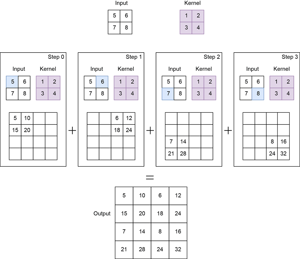
Figure 10.18 shows an example with input of shape 1 × 1 × 2 × 2. The kernel is of shape 1 × 1 × 2 × 2. Transpose convolution with stride 2 results in an output of shape 1 × 1 × 4 × 4.
NOTE Fully functional code for transpose convolution, executable via Jupyter Notebook, can be found at http://mng.bz/radD.
Listing 10.7 PyTorch code for upsampling using transpose convolutions
import torch

x = torch.tensor([                               ①
        [5., 6.],
        [7., 8.]
    ])

w = torch.tensor([                               ②
        [1., 2.],
        [3., 4.]
    ])

x = x.unsqueeze(0).unsqueeze(0)                  ③

w = w.unsqueeze(0).unsqueeze(0)                  ④

transpose_conv2d = torch.nn.ConvTranspose2d(     ⑤
    1, 1, kernel_size=2, stride=2, bias=False)

transpose_conv2d.weight = torch.nn.Parameter(w,  ⑥
                requires_grad=False)


with torch.no_grad():                            ⑦

    y = transpose_conv2d(x)                      ⑧
① Instantiates the input tensor
② Instantiates the weights of the kernel
③ Converts the input tensor to N × Cin × H × W = 1 × 1 × 2 × 2
④ Converts the kernel to Cin × Cout × kH × kW = 1 × 1 × 2 × 2
⑤ Instantiates the transpose convolution layer
⑥ Sets the kernel weights
⑦ Instructs PyTorch to not compute gradients since we currently don’t require them
⑧ Runs the transpose convolution. y is of shape 4 × 4.
10.6 Adding convolution layers to a neural network
Until now, we have been discussing convolution layers with custom weights that we set. While this gives us a conceptual understanding of how convolution works, in real neural networks, we do not set the convolution weights ourselves. Rather, we expect the weights to be learned from loss minimization via backpropagation, as described in chapters 8 and 9. We look at popular neural network architectures in the next chapter. But from a programming point of view, the most important thing to learn is how to add a convolution layer to a neural network. This is what we learn in the following section.
As part of setting up the neural network, we specify its dimensions but not the weights. We also initialize the weight values. The weight values are updated during the backpropagation (the loss.backward() call) somewhat behind the scene (although PyTorch allows us to view their values if we choose to).
10.6.1 PyTorch- Adding convolution layers to a neural network
Let’s see how a convolutional layer is implemented as part of a larger neural network in PyTorch (the full neural network architecture is discussed in detail in the next chapter):
-
A neural network typically subclasses the
torch.nn.Modulebase class and implements theforward()method. The layers of the neural network are instantiated in the__init__()function. -
torch.nn.Sequentialis used to chain multiple layers one after another. The output of the first layer is fed into the second layer, and so on. -
Each
torch.nn.Conv2d()represents a single convolutional layer. Our code snippet instantiates three such convolutional layers with other layers in between (details are covered in the next chapter).
Listing 10.8 PyTorch code for a sample convolutional neural network
import torch

class SampleCNN(torch.nn.Module):
    def __init__(self, num_classes):
        super(LeNet, self).__init__()
        self.nn = torch.nn.Sequential(           ①

            torch.nn.Conv2d(
                in_channels=1, out_channels=6,
                kernel_size=5, stride=1),        ②

                         ...

            torch.nn.Conv2d(
                in_channels=6, out_channels=16,
                kernel_size=5, stride=1),

                         ...

            torch.nn.Conv2d(
                in_channels=16, out_channels=120,
                kernel_size=5, stride=1),        ③

                        ...
        )

    def forward(self, x):                        ④
        out = self.nn(x)
        return out
① torch.nn.Sequential is used to chain a sequence of layers together.
② Instantiates the convolutional layer
③ Implements the forward pass
④ Runs the convolution
10.7 Pooling
Until now, we have seen how a convolution layer slides over an input image and generates an output feature map that contains important features that describe the image. We looked at this in 1D, 2D, and 3D settings. In a typical deep neural network, multiple such convolution layers are stacked one after another to recognize more and more complex structures in the image. (We talk more about this in the next chapter.) A major drawback of the convolution layer is that it is very sensitive to the location of the features in the input. Minor variations in the position of input features can result in a different output feature map. Such variations can occur in the real world due to camera angle changes, rotations, crops, objects being present at varying distances from the camera, and so on. How do we handle such variations and make the neural network more robust?
One way to do so is via downsampling. A lower-resolution version of the feature map still contains the important features but at a lower precision/granularity. So even if important features are present at slightly varying locations in higher-resolution feature maps, they will be more or less at the same location in the lower-resolution feature maps. This is also known as local translation invariance.
In convolution neural networks, the downsampling operation is performed by pooling layers. Pooling layers essentially slide a small filter across the entire image. At each filter location, they capture a summary of the local patch using a pooling operation. The two most popular types of pooling operations are as follows:
-
Max pooling—Calculates the maximum value for each patch
-
Average pooling—Calculates the average value for each patch
Figure 10.19 illustrates this in detail. The size of the output feature map depends on the kernel size and the stride of the pooling layer. For example, if we use a 2 × 2 kernel with a stride of 2, as in figures 10.19 and 10.20, the output feature map becomes half the size of the input feature map. Similarly, using a 3 × 3 kernel with stride = 3 makes the output feature map one-third the size.
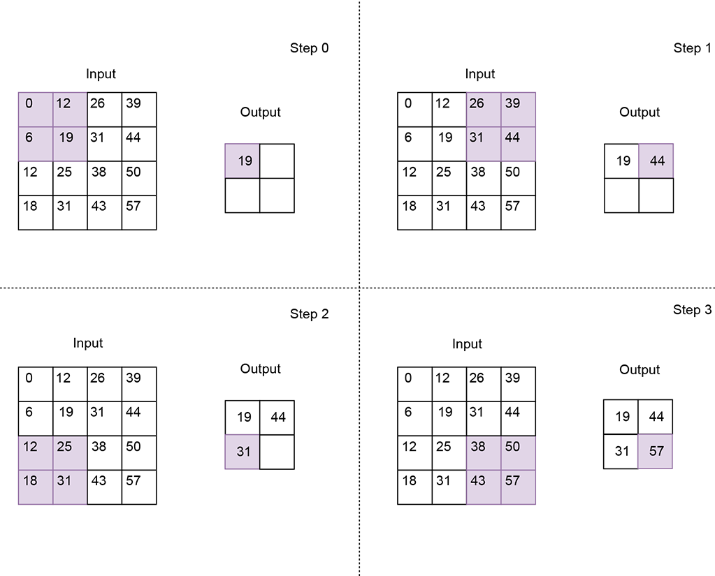
Figure 10.19 Max pooling using a 2 × 2 kernel with stride 2. The resulting output feature map is half the size of the input feature map. Each value of the output feature map is a max of the corresponding local patch in the input feature map.
Listing 10.9 PyTorch code for max and average pooling
import torch

X = torch.tensor([                ①
    [0, 12, 26, 39],
    [6, 19, 31, 44],
    [12, 25, 38, 50],
    [18, 31, 43, 57]
], dtype=torch.float32).unsqueeze(0).unsqueeze(0)

max_pool_2d = torch.nn.MaxPool2d( ②
    kernel_size=2, stride=2)

out_max_pool = max_pool_2d(X)     ③

avg_pool_2d = torch.nn.AvgPool2d( ④
    kernel_size=2, stride=2)

out_avg_pool = avg_pool_2d(X)     ⑤
① Instantiates a 4 × 4 input tensor
② Instantiates a 2 × 2 max pooling layer with stride 2
③ Output feature map is of size 2 × 2
④ Instantiates a 2 × 2 average pooling layer with stride 2
⑤ Output feature map is of size 2 × 2
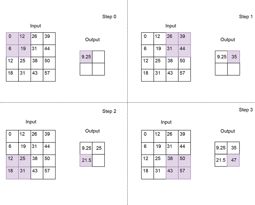
Figure 10.20 Average pooling using a 2 × 2 kernel with stride 2. The resulting output feature map is corresponding local patch in the input feature map.
Summary
In this chapter, we took an in-depth look at 1D, 2D, and 3D convolutions and their application to image and video analysis:
-
Convolutional layers help capture local patterns in input data because they connect only a small set of adjacent input values to an output value. This is different from the fully connected layers (aka linear layers) discussed in the previous chapters, where all inputs are connected to every output value.
-
A convolution operation involves sliding a kernel over an input array. It can conceptually be viewed as a matrix multiplication though it is not implemented this way for efficiency reasons). The kernel size, stride, and padding affect the size of the output.
-
The number of input elements over which the kernel slides upon completing a single step is known as stride.
-
As the kernel reaches the extremities of the input array, parts of it may fall outside the array. To deal with such cases, multiple padding strategies can be applied. In valid padding, the convolution operation stops when even a single kernel element falls outside the input array. In same (zero) padding, an input value of zero is assumed for all kernel elements that are outside the input array.
-
1D convolutions can conceptually be viewed as sliding a measuring ruler (1D kernel) across a stretched, straightened rope (1D input array). Real-world applications of 1D convolutions include smoothing and edge detection in curves.
-
2D convolutions can conceptually be viewed as sliding a tile (2D kernel) over the entire surface area of a wall (2D input array). Real-world applications of 2D convolutions include smoothing and edge detection in images.
-
3D convolutions can conceptually be viewed as sliding a brick (3D kernel) over the entire volume of a room 3D input array). Real-world applications of 3D convolutions include motion detection in an image sequence.
-
In transpose convolutions, the input array elements are multiplied by the kernel weights and then distributed across the output array. Real-world applications of transpose convolutions include upsampling, where lower-resolution inputs are converted into higher-resolution outputs. Autoencoders use transpose convolutions to reconstruct images from embeddings.
-
Pooling layers essentially slide a kernel across the input, capturing a summary of the local patch at each kernel location. They help improve the robustness of convolutional neural networks to minor variations in input features. The two most popular pooling operations are max pooling (calculates the maximum value of the local patch) and average pooling (calculates the average value of the local patch). Pooling layers result in downsampling of the input array. The output size depends on the size and stride of the pooling kernel.