11 Neural networks for image classification and object detection
This chapter covers
- Using deeper neural networks for image classification and object detection
- Understanding convolutional neural networks and other deep neural network architectures
- Correcting imbalances in neural networks
If a human is shown the image in figure 11.1, they can instantly recognize the objects in it, categorizing them as a bird, a plane, and Superman. In image classification, we want to impart this capability to computers—the ability to recognize objects in an image and classify them into one or more known and predetermined categories. Apart from identifying the object categories, we can also identify the location of the objects in the image. An object’s location can be described by a bounding box: a rectangle whose sides are parallel to coordinate axes. A bounding box is typically specified by four parameters: [(xtl, ytl),(xbr, ybr)], where (xtl, ytl) are the xy coordinates of the top-left corner and (xbr, ybr) are the xy coordinates of the bottom-right corner of the bounding
box. The problem of identifying and categorizing the objects present in the image is called image classification. If we also want to identify their location in the image, it is referred to as object detection. Image classification and object detection are some of the most fundamental problems in computer vision. While the human brain can both classify and localize objects in images almost intuitively, how do we train a machine to do this? Before deep learning, computer vision techniques involved hand-crafting image features (to encode color, edges, and shapes) and designing rules on top of these features to classify/localize objects. However, this is not a scalable approach because images are extremely complex and varied. Think of a simple object like an automobile. It can come in various sizes, shapes, and colors. It can be seen from afar or close (scales), from various viewpoints (perspectives), and on a cloudy day or a sunny day (lighting conditions). The car can be on a busy street or a mountain road backgrounds). It is nearly impossible to engineer features and rules that can handle all such variations.

Figure 11.1 Is it a bird? Is it a plane? Is it Superman?
Over the last 10 years, a new class of algorithms has emerged: convolutional neural networks (CNNs). They do not rely on hand-engineered features but instead learn the relevant features from data. These models have shown tremendous success in several computer vision tasks, achieving (and sometimes even surpassing) human-level accuracy. They are increasingly used in the industry for applications ranging from medical diagnostics to e-commerce to manufacturing. In this chapter, we detail some of the most popular deep neural network architectures used for image classification and object detection. We look at some of their salient features, take a deep dive into the architectural details to understand how and why they work, and apply them to real-world problems.
NOTE Fully functional code for this chapter, executable via Jupyter Notebook, can be found at http://mng.bz/vojq
11.1 CNNs for image classification: LeNet
In chapter 10, we discussed the convolution operation in 1D, 2D, and 3D scenarios. We also saw how to implement a single convolutional layer as part of a larger neural network. This section shows how a neural network with multiple convolutional layers can be used for image classification. (If needed, ou are encouraged to revisit chapter 10.) For this purpose, let’s consider the MNIST data set, a large collection of handwritten digits (0 through 9). It contains a training set of 60,000 images and a test set of 10,000 images. Each image is 28 × 28 in size and contains a center crop of a single digit. Figure 11.2 shows sample images from the MNIST data set.
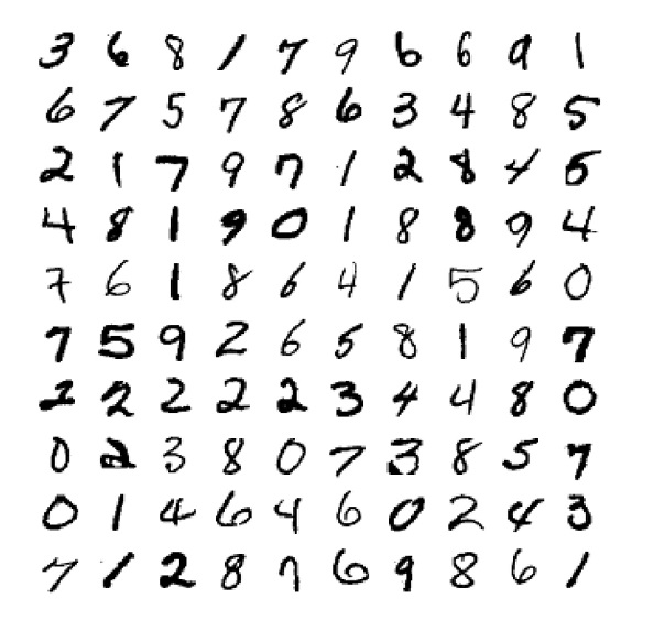
Figure 11.2 Sample images from the MNIST data set. (Source: “Gradient-based learning applied to document recognition”; http://mng.bz/Wz0a.)
We’d like to build a classifier that takes in a 28 × 28 image as input and emits a label from 0 to 9 based on the digit contained in the image. One of the most popular neural network architectures for this task is the LeNet, which was proposed by LeCun et al. in their 1998 paper, “Gradient-based learning applied to document recognition” (http://mng.bz/Wz0a). The LeNet architecture is illustrated in figure 11.3 (LeNet expects input images of size 32 × 32, so the 28 × 28 MNIST images are resized to 32 × 32 before being fed into the network):
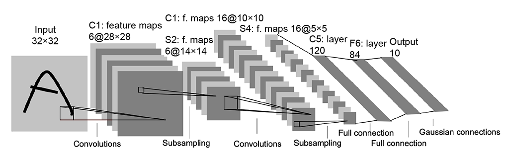
Figure 11.3 LeNet. (Source: “Gradient-based learning applied to document recognition”; http://mng.bz/Wz0a.)
-
It consists of three convolutional layers with 5 × 5 kernels convolved with a stride of 1. The first convolution layer produces 6 feature maps of size 28 × 28, the
second convolution layer produces 16 feature maps of size 10 × 10, and the third convolution layer produces 120 feature maps of size 1 × 1 which are flattened into a 120-dimensional vector)
-
The first two convolutional layers are followed by subsampling (aka pooling) layers, which perform a local averaging and subsampling of the feature map, thus reducing the resolution of the feature map and the sensitivity of the output to shifts and distortions in the input. A pooling kernel of size 2 × 2 is applied, reducing the feature map size to half its original size. Refer to section 10.7 for more about pooling.
-
Every feature map is followed by a tanh activation layer. This introduces nonlinearity into the network, increasing its expressive power because it can now model the output as a nonlinear combination of the inputs. If we did not have a nonlinear activation function, no matter how many layers we had, the neural network would still behave as a single-linear-layer network because the combination of multiple linear layers is just another linear layer. While the original LeNet paper used tanh as the activation function, several activation functions such as ReLU and sigmoid can also be used. ReLU is discussed in detail in section 11.2.1.1. Detailed discussions of sigmoid and tanh can be found in sections 8.1 and 8.1.2.
-
The output feature map is passed through two fully connected (FC, aka linear) layers, which finally produce a 10-dimensional logits vector that represents the score for every class. The logits scores are converted into probabilities using the softmax layer.
-
CrossEntropyLoss, discussed in section 6.3, is used to compute the difference between the predicted probabilities and the ground truth.
NOTE A feature map is a 2D array of points (that is, a grid) with a fixed-size vector associated with every point. An image is an example of a feature map, with each point being a pixel and the associated vector representing the pixel’s color. A convolution layer transforms an input feature map into an output feature map. The output feature map usually has smaller width and height but a longer per-point vector.
The LeNet performs very well on the MNIST data set, achieving test accuracies greater than 99%. A PyTorch implementation of LeNet is presented next.
11.1.1 PyTorch- Implementing LeNet for image classification on MNIST
NOTE Fully functional code for training the LeNet, executable via Jupyter Notebook, can be found at http://mng.bz/q2gz.
Listing 11.1 PyTorch code for the LeNet
import torch

class LeNet(torch.nn.Module):
    def __init__(self, num_classes):
        super(LeNet, self).__init__()
        self.conv1 = torch.nn.Sequential(
                        torch.nn.Conv2d(
                            in_channels=1, out_channels=6,     ①
                            kernel_size=5, stride=1),
                        torch.nn.Tanh(),                       ②
                        torch.nn.AvgPool2d(kernel_size=2))     ③
        self.conv2 = torch.nn.Sequential(
                        torch.nn.Conv2d(
                            in_channels=6, out_channels=16,
                            kernel_size=5, stride=1),
                        torch.nn.Tanh(),
                        torch.nn.AvgPool2d(kernel_size=2))
        self.conv3 = torch.nn.Sequential(
                        torch.nn.Conv2d(
                            in_channels=16, out_channels=120,
                            kernel_size=5, stride=1),
                        torch.nn.Tanh())
        self.fc1 = torch.nn.Sequential(
                        torch.nn.Linear(
                            in_features=120, out_features=84), ④
                        torch.nn.Tanh())
        self.fc2 = torch.nn.Linear(
            in_features=84, out_features=num_classes)          ⑤

    def forward(self, X):                                      ⑥
        conv_out = self.conv3(self.conv2(self.conv1(X)))
        batch_size = conv_out.shape[0]
        conv_out = conv_out.reshape(batch_size, -1)            ⑦
        logits = self.fc2(self.fc1(conv_out))                  ⑧
        return logits

    def predict(self, X):
        logits = self.forward(X)
        probs = torch.softmax(logits, dim=1)                   ⑨
        return torch.argmax(probs, 1)
① 5 × 5 conv
② Tanh activation
③ 2 × 2 average pooling
④ First FC layer
⑤ Second FC layer
⑥ X.shape: N × 3 × 32 × 32. N is the batch size.
⑦ conv_out.shape: N × 120 × 1 × 1
⑧ logits.shape: N × 10
⑨ Computes the probabilities using softmax
11.2 Toward deeper neural networks
The LeNet model is not a very deep network since it has only three convolutional layers. While this is sufficient to achieve accurate results on a simple data set like MNIST, it doesn’t work well on real-world image classification problems since it does not have enough expressive power to model complex images. So, we typically go for much deeper neural networks with multiple convolutional layers. Adding more layers does the following:
-
Brings extra expressive power due to extra nonlinearity—Since every layer brings with it a new set of learnable parameters and extra nonlinearity, a deeper network can model more complex relationships between input data elements. Lower layers typically learn simpler features of the object, like lines and edges, whereas higher layers learn more abstract features of the object, like shapes or sets of lines.
-
Achieves the same reach with fewer parameters—Let’s examine this via an example. Consider two output feature maps, one produced by a single 5 × 5 convolution on the input and another produced by two 3 × 3 convolutions applied one after another in sequence on the input. Assume a stride of 1 and the same (zero) padding. Figure 11.4 illustrates this scenario. Consider a single grid point in the output feature map. In both cases, the output value of the grid point is derived from a 5 × 5 patch in the input. We say the indicated 5 × 5 input patch is the receptive field of the output grid points. Thus, in both cases, the output grid point is a digest of the same input: that is, it expresses the same information. However, in the deeper network, there are fewer parameters. The number of parameters in a single 5 × 5 filter is 25, whereas that in two 3 × 3 filters is 2 × 9 = 18 (assuming a single channel input image). This is a 38% difference. Similarly, if we compare one 7 × 7 filter with three 3 × 3 filters, they have the same receptive field, but the 7 × 7 filter has 81% more parameters than the 3 × 3 filter.
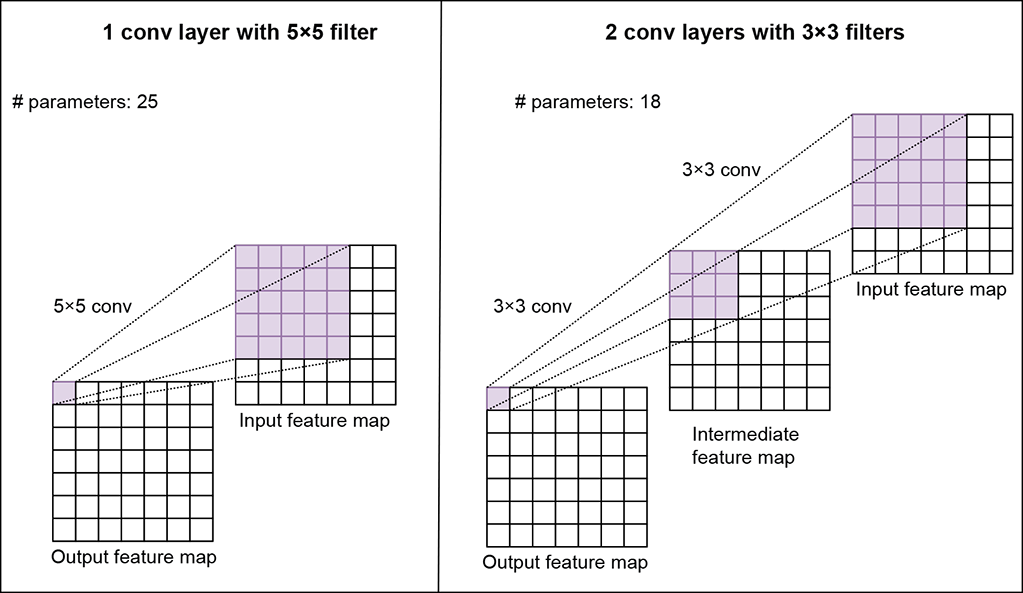
Figure 11.4 A single 5 × 5 convolution layer vs. two 3 × 3 convolution layers
Now, let’s look at some of the most popular deep convolutional networks used for image classification. The first deep network that reignited the deep learning revolution was AlexNet, which was published by Krizhevsky et al. in 2012. It significantly outperformed all previous state-of-the-art algorithms on the ImageNet Large Scale Visual Recognition Challenge (ILSVRC), a complex data set with 1.3 million images across 1,000 classes. Since AlexNet, several deep networks have improved on the previous state of the art, such as GoogleNet, VGG, and ResNet. In this chapter, we discuss the key concepts that make each of these networks work. For a detailed review of their architectures, training methodologies, and final results, you are encouraged to read the original papers linked in each section.
11.2.1 VGG (Visual Geometry Group) Net
The VGG family of networks was created by the Visual Geometry Group from the University of Oxford (https://arxiv.org/pdf/1409.1556.pdf). Their main contribution was a thorough evaluation of networks of increasing depth using an architecture with very small (3 × 3) convolution filters. They demonstrated that by using 3 × 3 convolutions and networks with 16–19 weight layers, they could outperform previous state-of-the-art results on the ILSVRC-2014 challenge. The VGG network had two main differences compared to prior works:
-
Use of smaller (3 × 3) convolution filters—Prior networks often relied on larger kernels of size 7 × 7 or 11 × 11 in the first convolution layers. VGG instead only used 3 × 3 kernels throughout the network. As discussed in section 11.2, three 3 × 3 filters have the same receptive field as a single 7 × 7 filter. So what does replacing the 7 × 7 filter with three smaller filters buy?
-
More nonlinearity and hence more expressive power because we have a ReLU activation function applied at the end of every convolution layer
-
Fewer parameters (49C2 vs. 27C2), which means faster learning and more robustness to overfitting
-
-
Removal of the local response normalization (LRN) layers—LRN was first introduced in the AlexNet architecture. Its purpose was twofold: to bound the output of the ReLU layer, which is an unbounded function and can produce outputs as large as the training permits; and to encourage lateral inhibition wherein a neuron can suppress the activity of its neighbors (this in effect acts as a regularization). The VGG paper demonstrated that adding LRN layers did not improve accuracy, so VGG chose to remove them from its architecture.
The VGG family of networks comes in five different configurations, which mainly differ in the number of layers (VGG-11, VGG-13, VGG-16, and VGG-19). Regardless of the exact configuration, the VGG family of networks follows a common structure. Here, we discuss these commonalities (a detailed description of the differences can be found in the original paper):
-
All architectures work on 224 × 224 input images.
-
All architectures have five convolutional blocks (conv blocks):
-
Each block can have multiple convolution layers followed by a max pool layer at the end.
-
All individual convolution layers use 3 × 3 kernels with a stride of 1 and same padding. Therefore, they don’t change the spatial resolution of the output feature map.
-
All convolution layers within a single conv block have the same-sized output feature maps.
-
Each convolution layer is followed by a ReLU layer that adds nonlinearity.
-
The max pool layer at the end of every conv block reduces the spatial resolution to half.
-
-
Since each conv block downsamples by 2, the input feature map is reduced 25 (32) times, resulting in an output feature map of size 7 × 7. Additionally, at each conv block, the number of feature maps is doubled.
-
All architectures end with three FC layers:
-
The first takes a 51,277-sized input and converts it into a 4,096-dimensional output.
-
The second takes the resulting 4,096-dimensional output and converts it into another 4,096-dimensional output.
-
The final takes the resulting 4,096-dimensional output and converts it into a C-dimensional output, where C stands for the number of classes. In the case of ImageNet classification, C is 1,000.
-
The architecture diagram for VGG-11 is shown in figure 11.5. The column on the left represents the shape of the input tensor to each layer. The column on the right represents the shape of the output tensor from each layer.
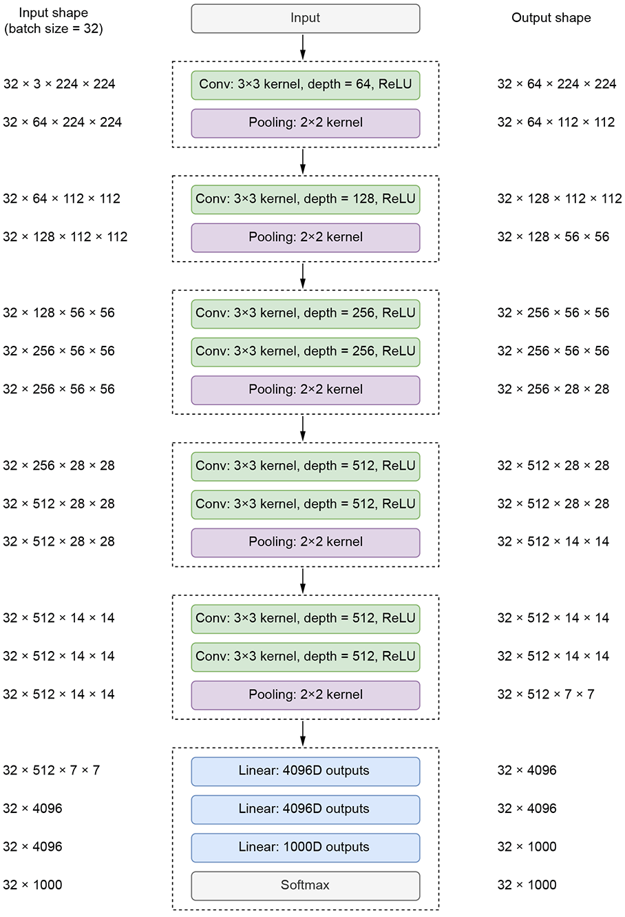
Figure 11.5 VGG-11 architecture diagram. All shapes are of the form N × C × H × W, where N is the batch size, C is the number of channels, H is the height, and W is the width.
ReLU nonlinearity
As we’ve discussed previously, nonlinear layers give the deep neural network more expressive power to model complex mathematical functions. In chapter 8, we looked at two nonlinear functions: sigmoid and tanh. However, the VGG network (like AlexNet) consists of a different nonlinear layer called rectified linear unit (ReLU). To understand the rationale for this choice, let’s revisit the sigmoid function and look at some of its drawbacks.
Figure 11.6 plots the sigmoid function along with its derivative. As the plot shows, the gradient (derivative) is maximum when the input is 0, and it quickly tapers down to 0 as the input increases/decreases. This is true for the tanh activation function as well. It means when the output of a neuron before the sigmoid layer) is either high or low, the gradient becomes small. While this may not be an issue in shallow networks, it becomes a problem in larger networks because the gradients can become too small for training to work effectively. Gradients of neural networks are calculated using backpropagation. By the chain rule, the derivatives of each layer are multiplied down the network, starting from the final layer and moving toward the initial layers. If the gradients at each layer are small, a small number multiplied by another small number is an even smaller number. Thus the gradients at the initial layers are very close to 0, making the training ineffective. This is known as the vanishing gradient problem.
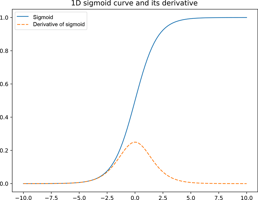
Figure 11.6 Graph of a 1D sigmoid function (dotted curve) and its derivative (solid curve)
The ReLU function addresses this problem. Figure 11.7 shows a graph of the ReLU function. Its equation is given by
ReLU(x) = max(0, x)
Equation 11.1
The derivative of ReLU is 1 (constant) when x is greater than 0, and 0 everywhere else. Therefore, it doesn’t suffer from the vanishing gradient problem. Most deep networks today use ReLU as their activation function. The AlexNet paper demonstrated that using ReLU nonlinearity significantly speeds up training because it helps with faster convergence.
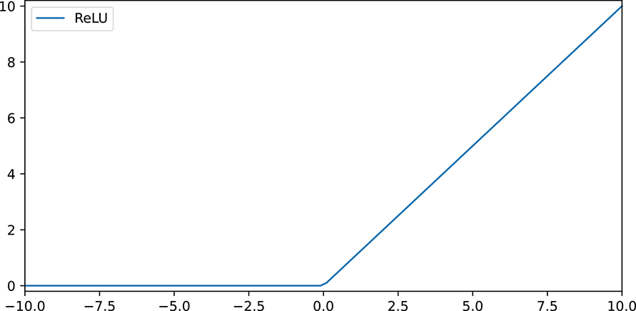
Figure 11.7 Graph of the ReLU function
PyTorch- VGG
Now let’s see how to implement the VGG network in PyTorch. First, let’s implement a single conv block, which is the core component of the VGG net. This conv block will later be repeated multiple times to form the entire VGG network.
NOTE Fully functional code for the VGG network, executable via Jupyter Notebook, can be found at http://mng.bz/7WE4.
Listing 11.2 PyTorch code for a convolutional block
class ConvBlock(nn.Module):
    def __init__(self, in_channels, num_conv_layers, num_features):
        super(ConvBlock, self).__init__()

        modules = []

        for i in range(num_conv_layers):
            modules.extend([
                nn.Conv2d(
                    in_channels, num_features,      ①
                    kernel_size=3, padding=1),      ②
                nn.ReLU(inplace=True)
            ])

            in_channels = num_features
        modules.append(nn.MaxPool2d(kernel_size=2)) ③
        self.conv_block = nn.Sequential(*modules)

    def forward(self, x):
        return self.conv_block(x)
① 3 × 3 conv
② ReLU nonlinearity
③ 2 × 2 max pooling
Next, let’s implement the convolutional backbone (conv backbone) builder, which allows us to create different VGG architectures via simple configuration changes.
Listing 11.3 PyTorch code for the conv backbone
class ConvBackbone(nn.Module):
    def __init__(self, cfg):                        ①


        super(ConvBackbone, self).__init__()

        self.cfg = cfg

        self.validate_config(cfg)

        modules = []
        for block_cfg in cfg:                       ②
            in_channels, num_conv_layers, num_features = block_cfg
            modules.append(ConvBlock(               ③
            in_channels, num_conv_layers, num_features))
        self.features = nn.Sequential(*modules)

    def validate_config(self, cfg):
        assert len(cfg) == 5 # 5  conv blocks
        for i, block_cfg in enumerate(cfg):
            assert type(block_cfg) == tuple and len(block_cfg) == 3
            if i == 0:
                assert block_cfg[0] == 3            ④
            else:
                assert block_cfg[0] == cfg[i-1][-1] ⑤

    def forward(self, x):
        return self.features(x)
① Cfg: [(in_channels, num_conv_layers, num_features),] The different VGG networks can be created without duplicating code by passing in the right cfg.
② Iterates over conv block configurations
③ Instantiates the conv block defined in listing 11.2
④ There must be three input channels.
⑤ out_Features of the previous block should be equal to in_features of the current block.
The conv backbone is instantiated with a config that contains the list of configurations for each of the conv blocks. The config for VGG-11 contains fewer layers, whereas that for VGG-19 contains more layers. The output of the conv backbone is fed into the classifier, which consists of three FC layers. Together, the conv backbone and the classifier form the VGG module.
Listing 11.4 PyTorch code for the VGG network
class VGG(nn.Module):
    def __init__(self, conv_backbone, num_classes):
        super(VGG, self).__init__()
        self.conv_backbone = conv_backbone   ①
        self.classifier = nn.Sequential(
            nn.Linear(512 * 7 * 7, 4096),
            nn.ReLU(True),
            nn.Dropout(),
            nn.Linear(4096, 4096),           ②
            nn.ReLU(True),
            nn.Dropout(),
            nn.Linear(4096, num_classes)
        )

    def forward(self, x):
        conv_features = self.conv_backbone(x)

        logits = self.classifier(
            conv_features.view(
                conv_features.shape[0], -1)) ③
        return logits
① Backbone network defined in listing 11.3
② The classifier is made up of three linear Layers. The first two are followed by ReLU nonlinearity.
③ Flattens the conv features before passing it to the classifier
A VGG-11 network can be instantiated as follows.
Listing 11.5 PyTorch code instantiating a VGG network from a specific config
vgg11_cfg = [                             ①
    (3, 1, 64),
    (64, 1, 128),
    (128, 2, 256),
    (256, 2, 512),
    (512, 2, 512)
]

vgg11_backbone = ConvBackbone(vgg11_cfg)  ①
num_classes = 1000
vgg11 = VGG(vgg11_backbone, num_classes)  ①
① Creates the cfg for VGG-11
② Instantiates the conv backbone
③ Instantiates the VGG network
While we have discussed how to implement VGG in PyTorch, we don’t do this in practice because the torchvision package already implements the VGG network, along with several other popular deep networks. It is recommended that you use the torchvision implementation, as shown here:
import torchvision
vgg11 = torchvision.models.vgg11()
11.2.2 Inception: Network-in-network paradigm
Previously, we saw how increasing the depth of a neural network—that is, the number of layers—can improve accuracy because it increases the expressive power of the network. Alternatively, we could increase the width of the network—the number of units at each level—to improve accuracy. However, both these methods suffer from two main drawbacks. First, blindly increasing the size of the network can lead to overfitting, wherein the network memorizes certain patterns in the training data that don’t extend well to test data. And second, increased computation resources are required during both training and inference times. The Inception architecture, introduced by Szegedy et al. in their paper "Going deeper with convolutions" (https://arxiv.org/pdf/1409.4842v1.pdf), aims to address both these drawbacks. The Inception architecture increases the network’s depth and width while keeping the computational budget constant. In this section, we examine the main idea behind the Inception architecture. While there have been several improvements to it Inception_v2, Inception_v3, Inception_ResNet, and so on), we discuss the original: Inception_v1.
Prior deep learning architectures typically stacked convolutional filters sequentially: each layer applied a set of convolutional filters of the same size and passed it to the subsequent layer. The kernel size of the filter at each layer depended on the architecture. But with such an architecture, how do we know we have chosen the right kernel size for each layer? If we are detecting a car, say, the fraction of the image area (that is, the number of pixels) occupied by the car is different in an image taken close up than in one taken from far away. We say the scale of the car object is different in the two images. Consequently, the number of pixels that must be digested to recognize the car will differ at different scales. A larger kernel is preferred for information at a larger scale, and vice versa. An architecture that is forced to choose one kernel size may not be optimal. The Inception module tackles this problem by having multiple kernels of different sizes at each level and taking weighted combinations of the outputs. The network can learn to weigh the appropriate kernel more than others. The naive implementation of the Inception module performs convolutions on the input using three kernel sizes: 1 × 1, 3 × 3, and 5 × 5. Max pooling is also performed, using a 3 × 3 kernel with stride 1 and padding 1 (for output and input to be the same size). The outputs are concatenated and sent into the next Inception module. See figure 11.8 for details.
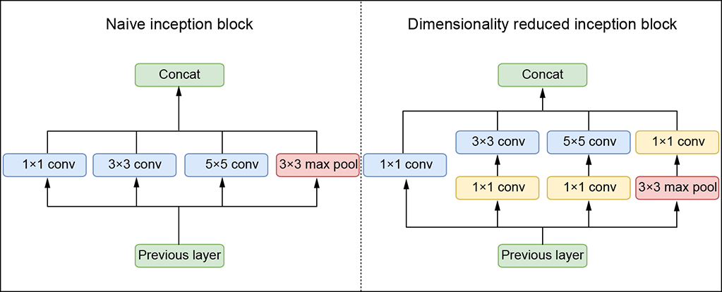
Figure 11.8 Inception_v1 architecture
This naive Inception block has a major flaw. Using even a small number of 5 × 5 filters can prohibitively increase the number of parameters. This becomes even more expensive when we add the pooling layer, where the number of output filters equals the number of filters in the previous stage. Thus, concatenating the output of the pooling layer with the outputs of convolutional layers would lead to an inevitable increase in the number of output features. To fix this, the Inception module uses 1 × 1 convolution layers before the 3 × 3 and 5 × 5 filters to reduce the number of input channels. This drastically reduces the number of parameters of the 3 × 3 and 5 × 5 convs. While it may seem counterintuitive, 1 × 1 convs are much cheaper than 3 × 3 and 5 × 5 convs. Additionally, 1 × 1 convolution is applied after pooling see figure 11.8).
A neural network architecture was built using the dimension-reduced Inception module and was popularly known as GoogLeNet. GoogLeNet has nine such Inception modules stacked linearly. It is 22 layers deep (27, including the pooling layers). It uses global average pooling at the end of the last Inception module. With such a deep network, there is always the vanishing gradient problem; to prevent the middle part of the network from “dying out,” the paper introduced two auxiliary classifiers. This is done by applying softmax to the output of two of the intermediate Inception modules and computing an auxiliary loss over the ground truth. The total loss function is a weighted sum of the auxiliary loss and the real loss. You are encouraged to read the original paper to understand the details.
PyTorch- Inception block
Let’s see how to implement an Inception block in PyTorch. We typically don’t do this in practice because end-to-end deep network architectures containing Inception blocks are already implemented in the torchvision package. However, we implement the Inception block from scratch to understand the details.
NOTE Fully functional code for the Inception block, executable via Jupyter Notebook, can be found at http://mng.bz/mxn0.
Listing 11.6 PyTorch code for a naive Inception block
class NaiveInceptionModule(nn.Module):
    def __init__(self, in_channels, num_features=64):
        super(NaiveInceptionModule, self).__init__()

        self.branch1x1 = torch.nn.Sequential(                   ①
                        nn.Conv2d(
                            in_channels, num_features,
                            kernel_size=1, bias=False),
                        nn.BatchNorm2d(num_features, eps=0.001),
                        nn.ReLU(inplace=True))

        self.branch3x3 = torch.nn.Sequential(
                        nn.Conv2d(                              ②
                            in_channels, num_features,
                            kernel_size=3, padding=1, bias=False),
                        nn.BatchNorm2d(num_features, eps=0.001),
                        nn.ReLU(inplace=True))

        self.branch5x5 = torch.nn.Sequential(                   ③
                        nn.Conv2d(
                            in_channels, num_features,
                            kernel_size=5, padding=2, bias=False),
                        nn.BatchNorm2d(num_features, eps=0.001),
                        nn.ReLU(inplace=True))

        self.pool = torch.nn.MaxPool2d(                         ④
            kernel_size=3, stride=1, padding=1)

    def forward(self, x):
        conv1x1 = self.branch1x1(x)
        conv3x3 = self.branch3x3(x)
        conv5x5 = self.branch5x5(x)
        pool_out = self.pool(x)
        out = torch.cat(                                        ⑤
            [conv1x1, conv3x3, conv5x5, pool_out], 1)
        return out
① 1 × 1 branch
② 3 × 3 branch
③ 5 × 5 branch
④ 3 × 3 pooling
⑤ Concatenates the outputs of the parallel branches
Listing 11.7 PyTorch code for a dimensionality reduced Inception block
class Inceptionv1Module(nn.Module):
    def __init__(self, in_channels, num_1x1=64,
                 reduce_3x3=96, num_3x3=128,
                 reduce_5x5=16, num_5x5=32,
                 pool_proj=32):
        super(Inceptionv1Module, self).__init__()

        self.branch1x1 = torch.nn.Sequential(
                        nn.Conv2d(               ①
                            in_channels, num_1x1,
                            kernel_size=1, bias=False),
                        nn.BatchNorm2d(num_1x1, eps=0.001),
                        nn.ReLU(inplace=True))

        self.branch3x3_1 = torch.nn.Sequential( ②
                        nn.Conv2d(
                            in_channels, reduce_3x3,
                            kernel_size=1, bias=False),
                        nn.BatchNorm2d(reduce_3x3, eps=0.001),
                        nn.ReLU(inplace=True))

        self.branch3x3_2 = torch.nn.Sequential(  ③
                        nn.Conv2d(
                            reduce_3x3, num_3x3,
                            kernel_size=3, padding=1, bias=False),
                        nn.BatchNorm2d(num_3x3, eps=0.001),
                        nn.ReLU(inplace=True))

        self.branch5x5_1 = torch.nn.Sequential(  ④
                        nn.Conv2d(
                            in_channels, reduce_5x5,
                            kernel_size=5, padding=2, bias=False),
                        nn.BatchNorm2d(reduce_5x5, eps=0.001),
                        nn.ReLU(inplace=True))
        self.branch5x5_2 = torch.nn.Sequential(  ⑤
                        nn.Conv2d(
                            reduce_5x5, num_5x5,
                            kernel_size=5, padding=2, bias=False),
                        nn.BatchNorm2d(num_5x5, eps=0.001),
                        nn.ReLU(inplace=True))

        self.pool = torch.nn.Sequential(         ⑥
                        torch.nn.MaxPool2d(
                            kernel_size=3, stride=1, padding=1),
                        nn.Conv2d(
                            in_channels, pool_proj,
                            kernel_size=1, bias=False),
                        nn.BatchNorm2d(pool_proj, eps=0.001),
                        nn.ReLU(inplace=True))


    def forward(self, x):
        conv1x1 = self.branch1x1(x)
        conv3x3 = self.branch3x3_2(self.branch3x3_1((x)))
        conv5x5 = self.branch5x5_2(self.branch5x5_1((x)))
        pool_out = self.pool(x)
        out = torch.cat(                         ⑦
            [conv1x1, conv3x3, conv5x5, pool_out], 1)
        return out
① 1 × 1 branch
② 1 × 1 conv in the 3 × 3 branch
③ 3 × 3 conv in the 3 × 3 branch
④ 1 × 1 conv in the 5 × 5 branch
⑤ 5 × 5 conv in the 5 × 5 branch
⑥ Max pooling followed by a 1 × 1 conv
⑦ Concatenates the outputs of the parallel branches
11.2.3 ResNet: Why stacking layers to add depth does not scale
We start with a fundamental question: is learning better networks as easy as stacking multiple layers? Consider the graphs in figure 11.9.
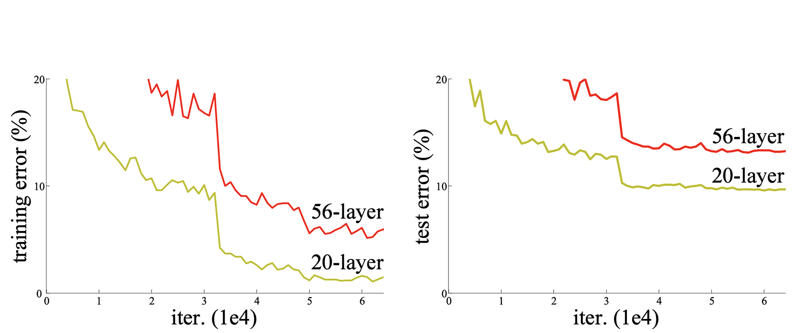
Figure 11.9 Training error (left) and test error (right) on the CIFAR-10 data set with 20-layer and 56-layer networks. (Source: “Deep residual learning for image recognition”; https://arxiv.org/pdf/1512.03385.pdf.)
This image from the ResNet paper “Deep residual learning for image recognition” (https://arxiv.org/pdf/1512.03385.pdf) shows the training and test error rates for two networks: a shallower network with 20 layers and a deeper network with 56 layers, on the CIFAR-10 data set. Surprisingly, the training and test errors are higher for the deeper (56-layer) network. This result is extremely counterintuitive because we expect deeper networks to have more expressive power and hence higher accuracies/lower error rates than their shallower counterparts. This phenomenon is referred to as the degradation problem: with the network depth increasing, the accuracy becomes saturated and degrades rapidly. We might attribute this to overfitting, but that is not the case because even the training errors are higher for the deeper network. Another cause could be vanishing/exploding gradients. However, the authors of the ResNet paper investigated the gradients at each layer and established that they are healthy (not vanishing/exploding). So, what causes the degradation problem, and how do we solve it?
Let’s consider a shallower architecture with n layers and a deeper counterpart that adds more layers to it (n + m layers). The deeper architecture should be able to achieve no higher loss than the shallow architecture. Intuitively, a trivial solution is to learn the exact n layers of the shallow architecture and the identity function for the additional m layers. The fact that this doesn’t happen in practice indicates that the neural network layers have a hard time learning the identity function. Thus the paper proposes "shortcut/skip connections" that enable the layers to potentially learn the identity function easily. This “identity shortcut connection” is the core idea of ResNet. Let’s look at a mathematical analogy. Let h(x) be the function we are trying to model (learn) via a stack of layers (not necessarily the entire network). It is reasonable to expect that the function g(x) = h(x) − x is simpler than h(x) and hence easier to learn. But we already have x at the input. So if we learn g(x) and add x to it to obtain h(x), we have effectively modeled h(x) by learning the simpler g(x) function. The name residual comes from g(x) = h(x) − x. Figure 11.10 shows this in detail.
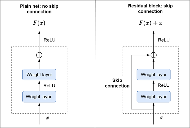
Figure 11.10 column shows a residual block with skip connections.
Now let’s revisit the earlier problem of degradation. We posited that normal neural network layers generally have difficulty learning the identity function. In the case of residual learning, to learn the identity function, h(x) = x, the layers need to learn g(x)=0. This can easily be done by driving all the layers’ weights to 0. Here is another way to think about it: if we initialize a regular neural network’s weights and biases to be 0 at the start, then every layer starts with the “zero” function: g(x) = 0. Thus, the output of every stack of layers with a shortcut connection, h(x) = g(x) + x, is already the identity function: h(x) = x when g(x) = 0.
In real cases, it is important to note that identity mappings are unlikely to be optimal: the network layers will want to learn actual features. In such cases, this reformulation isn’t preventing the network lawyers from doing so; the layers can still learn other functions like a regular stack of layers. We can think of this reformulation as preconditioning, which makes learning the identity function easier if needed. Additionally, by adding skip connections, we allow a direct path for the gradient to flow from layer to layer: the deeper layer has a direct path to x. This allows for better learning as information from the lower layers passes directly into the higher layers.
ResNet architecture
Now that we have seen the basic building block—a stack of convolutional (conv) layers with a skip connection—let’s delve deeper into the architecture of ResNet. ResNet architectures are constructed by stacking multiple building blocks on top of each other. They follow the same idea as VGG:
-
The convolutional layers mostly have 3 × 3 filters.
-
The layers have the same number of filters for a given output feature-map size.
-
If the feature-map size is halved, the number of filters is doubled to preserve the time complexity per layer.
ResNet uses conv layers with a stride of 2 to downsample, unlike VGG, which had multiple max pooling layers. The core architecture consists of the following components:
-
Five convolutional layer blocks—The first convolutional block consists of a 7 × 7 kernel with
stride=2,padding=3, andnum_features=64, followed by a max pooling layer with a 3 × 3 kernel,stride=2, andpadding=1. The feature map size is reduced from (224, 224) to (56, 56). The remaining convolutional blocksResidualConvBlock) are built by stacking multiple basic shortcut blocks together. Each basic block uses 3 × 3 filters, as described. -
Classifier—An average pooling block that runs on top of the conv block output, followed by a FC layer, which is used for classification.
You are encouraged to examine the diagrams in the original paper to understand the details. Now, let’s see how to implement a ResNet in PyTorch.
PyTorch- ResNet
In this section, we discuss how to implement a ResNet-34 from scratch. Note that this is seldom done in practice. The torchvision package provides ready-made implementations for all ResNet architectures. However, by building the network from scratch, we gain a deeper understanding of the architecture. First, let’s implement a basic skip connection block (BasicBlock) to see how the shortcut connection works.
NOTE Fully functional code for ResNet, executable via Jupyter Notebook, can be found at http://mng.bz/5K9q.
Listing 11.8 PyTorch code for BasicBlock
class BasicBlock(nn.Module):
    def __init__(self, in_channels, num_features, stride=1, downsample=None):
        super(BasicBlock, self).__init__()
        self.conv1 = nn.Sequential(                        ①

                        nn.Conv2d(
                            in_channels, num_features,
                            kernel_size=3, stride=stride, padding=1, bias=False),
                        nn.BatchNorm2d(num_features, eps=0.001),
                        nn.ReLU(inplace=True))
        self.conv2 = nn.Sequential(
                        nn.Conv2d(
                            num_features, num_features,
                            kernel_size=3, stride=1, padding=1, bias=False),
                        nn.BatchNorm2d(num_features, eps=0.001))


        self.downsample = downsample                       ②

        self.relu = nn.ReLU(inplace=True)


    def forward(self, x):
        conv_out = self.conv2(self.conv1(x))
        identity = x
        if self.downsample is not None:
            identity = self.downsample(x)
        assert identity.shape == conv_out.shape,
            f"Identity {identity.shape} and conv out {conv_out.shape} have different shapes"

        out = self.relu(conv_out + identity)               ③
        return out
① Instantiates two conv layers of filter size 3 × 3
② When input and output feature maps are not the same size, the input feature map is downsampled using a 1 × 1 convolution layer.
③ Creates a skip connection
Notice how the output of the residual block is a function of both the input and the output of the convolutional layer: ReLU(conv_out+x). This assumes that x and conv_out have the same shape. (Shortly, we discuss what to do when this isn’t the case.) Also note that adding the skip connections does not increase the number of parameters. The shortcut connections are parameter-free. This makes the solution cheap from a computational point of view and is one of the charms of shortcut connections.
Next, let’s implement a residual conv block consisting of a number of basic blocks stacked on top of each other. We have to handle two cases when it comes to basic blocks:
-
Case 1—Output feature map spatial resolution = Input feature map spatial resolution AND Number of output features = Number of input features. This is the most common case. Since there is no change in the number of features or the spatial resolution of the feature map, we can easily add the input and output via shortcut connections.
-
Case 2—Output feature map spatial resolution = 1/2 * Input feature map spatial resolution AND Number of output features = 2 * Number of input features. Remember that ResNet uses conv layers with a stride of 2 to downsample. The number of features is also doubled. This is done by the first basic block of every conv block except the second conv block). In this case, the input and output are not the same size. So how do we add them together as part of the skip connection? 1 × 1 convs are the answer. The spatial resolution of the input feature map is halved, and the number of input features is doubled by using a 1 × 1 conv with
stride=2andnum_features=2 * num_input_features.
Listing 11.9 PyTorch code for ResidualConvBlock
class ResidualConvBlock(nn.Module):
    def __init__(self, in_channels, num_blocks, reduce_fm_size=True):
        super(ResidualConvBlock, self).__init__()

        num_features = in_channels * 2 if reduce_fm_size else in_channels
        modules = []

        for i in range(num_blocks):                          ①
            if i == 0 and reduce_fm_size:
                stride = 2
                downsample = nn.Sequential(
                    nn.Conv2d(                               ②
                        in_channels, num_features,
                        kernel_size=1, stride=stride, bias=False),
                    nn.BatchNorm2d(num_features, eps=0.001),
                )
                basic_block = BasicBlock(
                    in_channels=in_channels, num_features=num_features,
                    stride=stride, downsample=downsample)
            else:
                basic_block = BasicBlock(
                    in_channels=num_features, num_features=num_features, stride=1)
            modules.append(basic_block)

        self.conv_block = nn.Sequential(*modules)


    def forward(self, x):
        return self.conv_block(x)
① The residual block is a stack of basic blocks.
② 1 × 1 convs to downsample the input feature map
With this, we are ready to implement ResNet-34.
Listing 11.10 PyTorch code for ResNet-34
class ResNet34(nn.Module):
    def __init__(self, num_basic_blocks, num_classes):
        super(ResNet, self).__init__()
        conv1 = nn.Sequential(                       ①
            nn.Conv2d(3, 64, kernel_size=7,
                stride=2, padding=3, bias=False),
            nn.BatchNorm2d(64, eps=0.001),
            nn.ReLU(inplace=True),
            nn.MaxPool2d(
                kernel_size=3, stride=2, padding=1)
        )


        assert len(num_basic_blocks) == 4            ②

        conv2 = ResidualConvBlock(                   ③
            in_channels=64, num_blocks=num_basic_blocks[0], reduce_fm_size=False)
        conv3 = ResidualConvBlock(
            in_channels=64, num_blocks=num_basic_blocks[1], reduce_fm_size=True)
        conv4 = ResidualConvBlock(
            in_channels=128, num_blocks=num_basic_blocks[2], reduce_fm_size=True)
        conv5 = ResidualConvBlock(
            in_channels=256, num_blocks=num_basic_blocks[3], reduce_fm_size=True)

        self.conv_backbone = nn.Sequential(*[conv1, conv2, conv3, conv4, conv5])

        self.avg_pool = nn.AdaptiveAvgPool2d((1, 1))
        self.classifier = nn.Linear(512, num_classes)


    def forward(self, x):
        conv_out = self.conv_backbone(x)
        conv_out = self.avg_pool(conv_out)
        logits = self.classifier(                    ④
            conv_out.view(conv_out.shape[0], -1))
        return logits
① Instantiates the first conv layer
② List of size 4, specifying the number of basic blocks per ResidualConvBlock
③ Instantiates four residual blocks
④ Flattens the conv feature before passing it to the classifier
As discussed earlier, we typically don’t implement our own ResNet. Instead, we use the ready-made implementation from the torchvision package like this:
import torchvision
resnet34 = torchvision.models.resnet34()  ①
① Instantiates resnet34 from the torchvision package
While we looked at the ResNet-34, there are deeper ResNet architectures like ResNet-50, ResNet-101, and ResNet-151 that use a different version of BasicBlock called BottleneckLayer. Similarly, there are several other variants inspired by ResNet, like ResNext, Wide ResNet, and so on. We don’t discuss these individual variants in this book because the core idea behind them remains the same. You are encouraged to read the original papers for a deeper understanding of the subject.
11.2.4 PyTorch Lightning
Let’s revisit the problem of digit classification that we looked at earlier. We primarily discussed the LeNet architecture and implemented it in PyTorch. Now, let’s implement the end-to-end code for training the LeNet model. Instead of doing it in vanilla PyTorch, we use the Lightning framework because it significantly simplifies the model development and training process.
Although PyTorch has all we need to train models, there’s much more to deep learning than attaching layers. When it comes to the actual training, we need to write a lot of boilerplate code, as we have seen in previous examples. This includes transferring data from CPU to GPU, implementing the training driver, and so on. Additionally, if we need to scale training/inferencing on multiple devices/machines, another set of integrations often needs to be done.
PyTorch Lightning is a solution that provides the APIs required to build models, data sets, and so on. It provides clean interfaces with hooks to be implemented. The underlying Lightning framework calls these hooks at appropriate points in the training process. The idea is that Lightning leaves the research logic to us while automating the rest of the boilerplate code. Additionally, Lightning brings in features like multi-GPU training, floating-point 16, and training on TPU inherently without requiring any code changes. More details about PyTorch Lightning can be found at https://www.pytorchlightning.ai/tutorials.
Training a model using PyTorch Lightning involves three main components: DataModule, LightningModule, and Trainer. Let’s see what each of these does.
DataModule
DataModule is a shareable, reusable class that encapsulates all the steps needed to process data. All data modules must inherit from LightningDataModule, which provides methods to be overridden. In this specific case, we will implement MNIST as a data module. This data module can now be used across multiple experiments spanning various models and architectures.
Listing 11.11 PyTorch code for an MNIST data module
class MNISTDataModule(LightningDataModule):
    DATASET_DIR = "datasets"

    def __init__(self, transform=None, batch_size=100):
        super(MNISTDataModule, self).__init__()
        if transform is None:
            transform = transforms.Compose(
                [transforms.Resize((32, 32)),
                transforms.ToTensor()])
        self.transform = transform
        self.batch_size = batch_size

    def prepare_data(self):                                  ①
        datasets.MNIST(root = MNISTDataModule.DATASET_DIR,
            train=True, download=True)
        datasets.MNIST(root=MNISTDataModule.DATASET_DIR,
            train=False, download=True)

    def setup(self, stage=None):
        train_dataset = datasets.MNIST(
            root = MNISTDataModule.DATASET_DIR, train=True,
            download=False, transform=self.transform)
        self.train_dataset, self.val_dataset = random_split( ②
            train_dataset, [55000, 5000])

        self.test_dataset = datasets.MNIST(
            root = MNISTDataModule.DATASET_DIR, train = False,
            download = False, transform=self.transform)

    def train_dataloader(self):                              ③
        return DataLoader(
            self.train_dataset, batch_size=self.batch_size,
            shuffle=True, num_workers=0)

    def val_dataloader(self):                                ④
        return DataLoader(
            self.val_dataset, batch_size=self.batch_size,
            shuffle=False, num_workers=0)

    def test_dataloader(self):                               ⑤
        return DataLoader(
            self.test_dataset, batch_size=self.batch_size,
            shuffle=False, num_workers=0)

    @property
    def num_classes(self):                                   ⑥
        return 10
① Download, tokenizes, and prepares the raw data
② Splits the training data set into training and validation sets
③ Creates the train data loader, which provides a clean interface for iterating over the data set. It handles batching, shuffling, and fetching data via multiprocessing, all under the hood.
④ Creates the val data loader
⑤ Creates the test data loader
⑥ Number of object categories in the data set
LightningModule
LightningModule essentially groups all the research code into a single module, making it self-contained. Notice the clean separation between DataModule and LightningModule—this makes it easy to train/evaluate the same model on different data sets. Similarly, different models can be easily trained/evaluated on the same data set.
A Lightning module consists of the following:
-
A model or system of models defined in the
initmethod -
A training loop defined in
training_step -
A validation loop defined in
validation_step -
A testing loop defined in
testing_step -
Optimizers and schedulers defined in
configure_optimizers
Let’s see how we can define the LeNet classifier as a Lightning module.
Listing 11.12 PyTorch code for LeNet as a Lightning module
class LeNetClassifier(LightningModule):

    def __init__(self, num_classes):                 ①

        super(LeNetClassifier, self).__init__()
        self.save_hyperparameters()

        self.conv1 = torch.nn.Sequential(
                        torch.nn.Conv2d(
                            in_channels=1, out_channels=6,
                            kernel_size=5, stride=1),
                        torch.nn.Tanh(),

                        torch.nn.AvgPool2d(kernel_size=2))
        self.conv2 = torch.nn.Sequential(
                        torch.nn.Conv2d(
                            in_channels=6, out_channels=16,
                            kernel_size=5, stride=1),
                        torch.nn.Tanh(),
                        torch.nn.AvgPool2d(kernel_size=2))
        self.conv3 = torch.nn.Sequential(
                        torch.nn.Conv2d(
                            in_channels=16, out_channels=120,
                            kernel_size=5, stride=1),
                        torch.nn.Tanh())
        self.fc1 = torch.nn.Sequential(
                        torch.nn.Linear(in_features=120, out_features=84),
                        torch.nn.Tanh())
        self.fc2 = torch.nn.Linear(in_features=84,
            out_features=num_classes)

        self.criterion = torch.nn.CrossEntropyLoss() ②

        self.accuracy = torchmetrics.Accuracy()

    def forward(self, X):                            ③
        conv_out = self.conv3(
            self.conv2(self.conv1(X)))
        batch_size = conv_out.shape[0]
        conv_out = conv_out.reshape(
            batch_size, -1)
        logits = self.fc2(self.fc1(conv_out))
        return logits                                ④

    def predict(self, X):                            ⑤
        logits = self.forward(X)
        probs = torch.softmax(logits, dim=1)
        return torch.argmax(probs, 1)

    def core_step(self, batch):                      ⑥
        X, y_true = batch
        y_pred_logits = self.forward(X)
        loss = self.criterion(y_pred_logits, y_true)
        accuracy = self.accuracy(y_pred_logits, y_true)
        return loss, accuracy

    def training_step(self, batch, batch_idx):       ⑦

        loss, accuracy = self.core_step(batch)
        if self.global_step \% 100 == 0:
            self.log("train_loss", loss, on_step=True, on_epoch=True)
            self.log("train_accuracy", accuracy, on_step=True, on_epoch=True)
        return loss

    def validation_step(self, batch,
        batch_idx, dataset_idx=None):                ⑧
        return self.core_step(batch)

    def validation_epoch_end(self, outputs):         ⑨
        avg_loss = torch.tensor([x[0] for x in outputs]).mean()
        avg_accuracy = torch.tensor([x[1] for x in outputs]).mean()
        self.log("val_loss", avg_loss)
        self.log("val_accuracy", avg_accuracy)
        print(f"Epoch {self.current_epoch},
            Val loss: {avg_loss:0.2f}, Accuracy: {avg_accuracy:0.2f}")
        return avg_loss

    def configure_optimizers(self):                  ⑩
        return torch.optim.SGD(model.parameters(), lr=0.01,
                      momentum=0.9)


    def checkpoint_callback(self):                   ⑪
        return ModelCheckpoint(monitor="val_accuracy", mode="max", save_top_k=1)
① In the init method, we typically define the model, the criterion, and any other setup steps required for training the model.
② Instantiates cross-entropy loss
③ Implements the model’s forward pass. In this case, the input is a batch of images, and the output is the logits. X.shape: [batch_size, C, H, W].
④ Logits.shape: [batch_size, num_classes]
⑤ Runs the forward pass, performs softmax to convert the resulting logits into probabilities, and returns the class with the highest probability
⑥ Abstracts out common functionality between the training and test loops, including the running forward pass, computing loss, and accuracy
⑦ Implements the basic training step: run forward pass, compute loss, accuracy. Logs any necessary values and returns the total loss.
⑧ Called at the end of all test steps for each epoch. The output of every test step is available via outputs. Here we compute the average test loss and accuracy by averaging across all test batches.
⑨ Implements the basic validation step: run forward pass, compute loss and accuracy, return them.
⑩ Configures the SGD optimizer
⑪ Implements logic to save the model. We save the model with the best val accuracy.
The model is independent of the data. This allows us to potentially run the LeNetClassifier model on other data modules without any code changes. Note that we are not doing the following steps:
-
Moving the data to a device
-
Calling
loss.backward -
Calling
optimizer.backward -
Setting
model.train()oreval() -
Resetting the gradients
-
Implementing the trainer loop
All of these are taken care of by PyTorch Lightning, thus eliminating a lot of boilerplate code.
Trainer
We are ready to train our model, which can be done using the Trainer class. This abstraction achieves the following:
-
We maintain control over all aspects via PyTorch code without an added abstraction.
-
The trainer uses best practices embedded by contributors and users from top AI labs.
-
The trainer allows us to override any key part that we don’t want automated.
Listing 11.13 PyTorch code for Trainer
dm = MNISTDataModule()                               ①
model = LeNetClassifier(num_classes=dm.num_classes)  ②
exp_dir = "/tmp/mnist"
trainer = Trainer(                                   ③
        default_root_dir=exp_dir,
        callbacks=[model.checkpoint_callback()],
        gpus=torch.cuda.device_count(), # Number of GPUs to run on
        max_epochs=10,
        num_sanity_val_steps=0
    )
trainer.fit(model, dm)                               ④
① Instantiates the data set
② Instantiates the model
③ Instantiates the trainer
④ Trains the model
Note that we do not write the trainer loop: we just call trainer.fit to train the model. Additionally, the logging automatically enables us to look at the loss and accuracy curves via TensorBoard.
Listing 11.14 PyTorch code for inferencing a model
X, y_true = (iter(dm.test_dataloader())).next()
with torch.no_grad():
    y_pred = model.predict(X) ①
① Runs model.predict()
To run inferencing using the trained model, we run model.predict on the input.
11.3 Object detection: A brief history
Until now, we have discussed the classification problem wherein we categorize an image as 1 of N object categories. But in many cases, this is not sufficient to truly describe an image. Consider figure 11.11—a very realistic image with four animals standing one on top of another, posing for the camera. It would be useful to know the object categories of each of the animals and their location (bounding-box coordinates) in the image. This is referred to as the object detection/localization problem. So, how do we localize objects in images?
Let’s say we could extract regions in the image so that each region contained only one object. We could then run an image classifier deep neural network (which we looked at earlier) to classify each region and select the regions with the highest confidence. This was the approach adopted by one of the first deep learning-based object detectors, a region-based CNN (R-CNN; https://arxiv.org/pdf/1311.2524.pdf). Let’s look at this in more detail.
11.3.1 R-CNN
The R-CNN approach to object detection consists of three main stages:
-
Selective search to identify regions of interest—This step uses a computer vision-based algorithm capable of extracting candidate regions. We do not go into the details of the selective search; you are encouraged to go through the original paper to understand the details. Selective search generates around 2,000 region proposals per image.
-
Feature extraction—A deep convolution neural network extracts features from each region of interest. Since deep neural networks typically take in fixed-sized inputs, the regions (which could be arbitrarily sized) are warped into a fixed size before being fed into the deep neural network.
-
Classification/Localization—A class-specific support vector machine (SVM) is trained on the extracted features to classify the region. Additionally, bounding-box regressors are added to fine-tune the object’s location within the region. During training, each region is assigned a ground-truth (GT) class based on its overlap with GT boxes. It is assigned a positive label if there is a high overlap and a negative label otherwise.
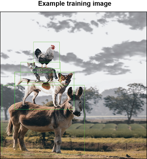
Figure 11.11 An image with multiple objects of different shapes and sizes
11.3.2 Fast R-CNN
One of the biggest disadvantages of the R-CNN-based approach is that we have to extract features for every region proposal independently. So, if we generate 2,000 proposals for a single image, we have to run 2,000 forward passes to extract the region features. This is prohibitively expensive and extremely slow (during both training and inference). Additionally, training is a multistage pipeline—selective search, the deep network, the SVMs on top of the features, and the bounding-box regressors—that is cumbersome to train and inference. To solve these problems, the authors of the R-CNN introduced a new technique called a Fast R-CNN https://arxiv.org/pdf/1504.08083.pdf). It significantly improved speeds: it is 9× faster than the R-CNN during training and 213× faster at test time. Additionally, it improves the quality of object detection.
Fast R-CNN makes two major contributions:
-
Region of interest (RoI) pooling—As mentioned, one of the fundamental issues with R-CNN is the need for multiple forward passes to extract the features for the region proposals of a single image. Instead, can we extract the features in one go? This problem is solved using RoI pooling. The Fast R-CNN uses the entire image as the input to the CNN instead of a single region proposal. Then, the RoIs (region proposal bounding boxes) are used on top of the CNN output to extract the region features in one pass. We will go into the details of RoI pooling as part of our Faster R-CNN discussion.
-
Multitask loss—The Fast R-CNN eliminates the need to use SVMs. Instead, the deep neural network does both classification and bounding-box regression. Unlike R-CNN, which only uses deep networks for feature extraction, the Fast R-CNN is more end-to-end. It is a single architecture for region proposal feature extraction, classification, and regression.
The high-level algorithm is as follows:
-
Use selective search to generate 2,000 region proposals/RoIs per image.
-
In a single pass of the Fast R-CNN, extract all the RoI features in a single pass using RoI pooling and then classify and localize objects using the classification and regression heads.
Since the feature extraction for all the region proposals happens in one pass, this approach is significantly faster than the R-CNN, where every proposal needs a separate forward pass. Additionally, since the neural network is trained end to end—that is, asked to do classification and regression—the accuracy of object detection is also improved.
11.3.3 Faster R-CNN
Why settle for fast when we can be faster? The Fast R-CNN was significantly faster than the R-CNN. However, it still needed selective search to be run to obtain region proposals. The selective-search algorithm can only be run on CPUs. Additionally, the algorithm is slow and time-consuming. Thus it became a bottleneck. Is there a way to get rid of selective search?
The obvious idea to consider is using deep networks to generate region proposals. This is the core idea of Faster R-CNN (FRCNN; https://arxiv.org/pdf/1506.01497.pdf): it eliminates the need for selective search and lets a deep network learn the region proposals. It was one of the first near-real-time object detectors. Since we are using a deep network to learn the region proposals, the region proposals are also better. Thus the resulting accuracy of the overall architecture is also much better.
We can view the FRCNN as consisting of two core modules:
-
Region proposal network (RPN)—This is the module responsible for generating the region proposals. RPNs are designed to efficiently predict region proposals with a wide range of scales and aspect ratios.
-
R-CNN module—This is the same as the Fast R-CNN. It receives a bunch of region proposals and performs RoI pooling followed by classification and regression.
Another important thing to note is that the RPN and the R-CNN module share the same convolutional layers: the weights are shared rather than learning two separate networks. In the next section, we discuss the Faster R-CNN in detail.
11.4 Faster R-CNN: A deep dive
Figure 11.12 shows the high-level architecture of the FRCNN. The convolutional layers (which we also call the convolutional backbone) extract feature maps from the input image. The RPN operates on these feature maps and emits candidate RoIs. The RoI pooling layer generates a fixed-sized feature vector for each region of interest and passes it on to a set of FC layers that emit softmax probability estimates over K object classes (plus a catch-all “background” class) and four numbers representing the bounding-box coordinates for each of the K classes. Let’s look at each of the components in more detail.
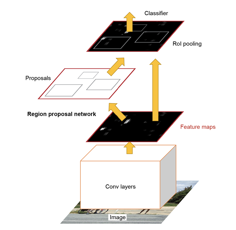
Figure 11.12 architecture. (Source: “Faster R-CNN: Toward real-time proposal networks”; https://arxiv.org/abs/1506.01497.)
11.4.1 Convolutional backbone
In the original implementation, the FRCNN used the convolution layers of VGG-16 as the convolutional backbone for both the RPN and the R-CNN modules. There has been one minor modification: the last pooling layer after the fifth convolution layer (conv5) is removed. As we’ve discussed regarding VGG architectures earlier, VGG reduces the spatial size of the feature map by 2 in every conv block via max pooling. Since the last pooling layer is removed, the spatial size is reduced by a factor of 24 = 16. So a 224 × 224 image is reduced to a 14 × 14 feature map at the output. Similarly, an 800 × 800 image would be reduced to a 50 × 50 feature map.
11.4.2 Region proposal network
The RPN takes in an image (of any arbitrary size) as input and emits a set of rectangular proposals that could potentially contain objects as output. The RPN operates on top of the convolutional feature map output by the last shared convolution layer. With the VGG backbone, an input image of size (h, w) is scaled down to (h/16, w/16). So each 16 × 16 spatial region in the input image is reduced to a single point on the convolutional feature map. Thus each point in the output convolutional feature map represents a 16 × 16 patch in the input image. The RPN operates on top of this feature map. Another subtle point to remember is that while each point in the convolutional feature map is chosen to correspond to a 16 × 16 patch, it has a significantly larger receptive field (the region in the input feature map that a particular output feature is affected by). The embedding at each point in the feature map is thus, in effect, the digest of a large receptive field.
Anchors
A key aspect of the object-detection problem is the variety of object sizes and shapes. Objects can range from very small (cats) to very large elephants). Additionally, objects can have different aspect ratios. Some objects may be wide, some may be tall, and so on. A naive solution is to have a single neural network detector head capable of identifying and recognizing all these objects of varying sizes and shapes. As you can imagine, this would make the job of the neural network detector extremely complex. A simpler solution is to have a wide variety of neural network detector heads, each responsible for solving a much simpler problem. For example, one head will only focus on large, tall objects and will only fire when such objects are present in the image. The other heads will focus on other sizes and aspect ratios. We can think of each head as being responsible for doing a single simple job. This type of setup greatly aids and benefits learning.
This was the intuition behind the introduction of anchors. Anchors are like reference boxes of varying shapes and sizes. All proposals are made relative to anchors. Each anchor is uniquely characterized by its size and aspect ratio and is tasked with detecting similarly shaped objects in the image. At each sliding-window location, we have multiple anchors spanning different sizes and aspect ratios. The original FRCNN architecture supported nine anchor configurations spanning three sizes and three aspect ratios, thus supporting a wide variety of shapes. These correspond to anchor boxes of scales (8, 16, 32) and aspect ratios (0.5, 1.0, and 2.0), respectively (see figure 11.13). Anchors are now ubiquitous across object detectors.
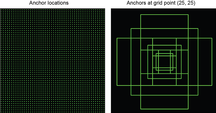
Figure 11.13 The left column shows the various grid-point locations on the output convolution feature original implementation) anchors across multiple sizes and aspect ratios. The right column shows the various anchors at a particular grid point.
NOTE Fully functional code for generating anchors, executable via Jupyter Notebook, can be found at http://mng.bz/nY48.
Listing 11.15 PyTorch code to generate anchors at a particular grid point
def generate_anchors_at_grid_point(
    ctr_x, ctr_y, subsample, scales, aspect_ratios):
    anchors = torch.zeros(
        (len(aspect_ratios) * len(scales), 4), dtype=torch.float)

    for i, scale in enumerate(scales):
        for j, aspect_ratio in enumerate(aspect_ratios): ①


            w = subsample * scale * torch.sqrt(aspect_ratio)
            h = subsample * scale * torch.sqrt(1 / aspect_ratio)


            xtl = ctr_x - w / 2                          ②
            ytl = ctr_y - h / 2
            xbr = ctr_x + w / 2
            ybr = ctr_y + h / 2

            index = i * len(aspect_ratios) + j
            anchors[index] = torch.tensor([xtl, ytl, xbr, ybr])
    return anchors
① Generates the height and width for different scales and aspect ratios
② Generates a bounding box centered around ctr_x, ctr_y) with width w, and height h
Listing 11.16 PyTorch code to generate all anchors for a given image
 def generate_all_anchors(                       ①


     input_img_size, subsample, scales, aspect_ratios):

    _, h, w = input_img_size

    conv_feature_map_size = (h//subsample, w//subsample)

    all_anchors = []                             ②


    ctr_x = torch.arange(
        subsample/2, conv_feature_map_size[1]*subsample+1, subsample)
    ctr_y = torch.arange(
        subsample/2, conv_feature_map_size[0]*subsample+1, subsample)

    for y in ctr_y:
        for x in ctr_x:
            all_anchors.append(
                generate_anchors_at_grid_point(  ③
                    x, y, subsample, scales, aspect_ratios))

    all_anchors = torch.cat(all_anchors)
    return all_anchors


input_img_size = (3, 800, 800)                   ④
c, height, width = input_img_size
scales = torch.tensor([8, 16, 32], dtype=torch.float)
aspect_ratios = torch.tensor([0.5, 1, 2])
subsample = 16
anchors = generate_all_anchors(input_img_size, subsample, scales, aspect_ratios)
① This isn’t the most efficient way to generate anchors. We’ve written simple code to ease understanding.
② Generates anchor boxes centered at every point in the conv feature map, which corresponds to a 16 × 16 (subsample, subsample) region in the input
③ Uses a function defined in listing 11.15
④ Defines config parameters and generates anchors
The RPN slides a small network over the output convolution feature map. The small network operates on an n × n spatial window of the convolution feature map. At each sliding-window location, it generates a lower-dimensional feature vector (512 dimensions for VGG) that is fed into a box-regression layer (reg) and a box-classification layer (cls). For each of the anchor boxes centered at that sliding window location, the classifier predicts objectness: a value from 0 to 1, where 1 indicates the presence of the object and the regressor predicts the region proposal relative to the anchor box. This architecture is naturally implemented with an n × n convolutional layer followed by two sibling 1 × 1 convolutional layers (for reg and cls), respectively. The original implementation in the FRCNN paper uses n = 3, which results in an effective receptive field of 228 pixels when using the VGG backbone. Figure 11.14 illustrates this in detail. Note that this network consists of only convolutional layers. Such an architecture is called a fully convolutional network FCN). FCNs do not have an input size restriction. Because they
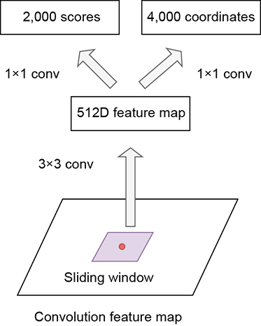
Figure 11.14 RPN architecture. From each sliding window, a 512-dimensional feature vector is generated using 3 × 3 convs. A 1 × 1 conv layer (classifier) takes the 512-dimensional feature Similarly, another 1 × 1 conv layer (regressor) generates 4k bounding-box coordinates from the 512-dimensional feature vector.
consist of only convolution layers, they can work with arbitrary-sized inputs. In the FCN, the combination of the n × n and 1 × 1 layers is equivalent to applying an FC layer over every embedding at each point in the convolutional feature map. Also, because we are convolving a convolutional network on top of the feature map to generate the regression and classification scores, the convolutional weights are common/shared across different positions on the feature map. This makes the approach translation invariant. A cat at the top of the image and a cat at the bottom of the image are picked up by the same anchor configuration (scale, aspect ratio) if they are similarly sized.
NOTE Fully functional code for the fully convolutional network of the RPN, executable via Jupyter Notebook, can be found at http://mng.bz/nY48.
Listing 11.17 PyTorch code for the FCN of the RPN
class RPN_FCN(nn.Module):

    def __init__(self, k, in_channels=512):  ①
        super(RPN_FCN, self).__init__()
        self.conv = nn.Sequential(
            nn.Conv2d(
                in_channels, 512, kernel_size=3,
                stride=1, padding=1),
            nn.ReLU(True))
        self.cls = nn.Conv2d(512, 2*k, kernel_size=1)
        self.reg = nn.Conv2d(512, 4*k, kernel_size=1)


    def forward(self, x):
        out = self.conv(x)                   ②

        rpn_cls_scores = self.cls(out).view( ③
            x.shape[0], -1, 2)
        rpn_loc = self.reg(out).view(        ④
            x.shape[0], -1, 4)

        ⑤
       return rpn_cls_scores       ,rpn_loc  ⑥
① Instantiates the small network that is convolved over the output conv feature map. It consists of a 3 × 3 conv layer followed by a 1 × 1 conv layer for classification and another 1 × 1 conv layer for regression.
② Output of the backbone: a convolutional feature map of size (batch_size, in_channels, h, w)
③ Converts (batch_size, h, w, 2k) to batch_size, h*w*k, 2)
④ Converts (batch_size, h, w, 4k) to batch_size, h*w*k, 4)
⑤ (batch_size, num_anchors, 2) tensor representing the classification score for each anchor box
⑥ (batch_size, num_anchors, 4) tensor representing the box coordinates relative to the anchor box
Generating GT for an RPN
So far, we have generated many anchor bounding boxes and a neural network capable of generating the classification and regression offsets for every anchor. While training the RPN, we need to provide a target GT) that both the classifier and regressor should predict for each anchor box. To do so, we need to look at the objects in the image and assign them to relevant anchors that contain the object. The idea is as follows: out of the thousands of anchors, the anchors that contain most of the object should try predicting and localizing the object. We saw earlier that the intuition behind creating anchors was to ensure that each anchor is responsible for one particular type of object shape, aspect ratio). Thus it makes sense that only anchors that contain the object are responsible for classifying it.
To measure whether the object lies within the anchor, we rely on intersection over union (IoU) scores. The IoU between two bounding boxes is defined as (area of overlap)/(area of union). So, if the two bounding boxes are very similar, their overlap is high, and their union is close to the overlap, resulting in a high IoU. If the two bounding boxes are varied, then their area of overlap is minimal, resulting in a low IoU (see figure 11.15).
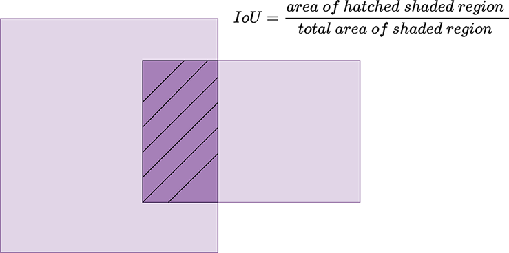
Figure 11.15 section of the two areas divided by the union of the two areas.
FRCNN provides some guidelines for assigning labels to the anchor boxes:
-
We assign a positive label 1 (which represents an object being present in the anchor box) to two kinds of anchors:
-
The anchor(s) with the greatest IoU overlap with a GT box
-
An anchor that has an IoU overlap greater than 0.7 with the GT box
-
-
We assign a negative label 0 (which represents no object being present in the anchor box, implying that it contains only background) to a non-positive anchor if its IoU ratio is less than 0.3 for all GT boxes.
-
Anchors that are neither positive nor negative do not contribute to the training objective.
Note that a single GT object may assign positive labels to multiple anchors. These outputs must be suppressed later to prevent duplicate detections (we discuss this in the subsequent sections). Also, any anchor box that lies partially outside the image is ignored.
NOTE Fully functional code for assigning GT labels to anchor boxes, executable via Jupyter Notebook, can be found at http://mng.bz/nY48.
Listing 11.18 PyTorch code to assign GT labels for each anchor box
valid_indices = torch.where(
    (anchors[:, 0] >=0) &
    (anchors[:, 1] >=0) &
    (anchors[:, 2] <=width) &                         ①
    (anchors[:, 3] <=height))[0]

rpn_valid_labels = -1 * torch.ones_like(              ②
    valid_indices, dtype=torch.int)

valid_anchor_bboxes = anchors[valid_indices]          ③

ious = torchvision.ops.box_iou(                       ④
    gt_bboxes, valid_anchor_bboxes)

assert ious.shape == torch.Size(
    [gt_bboxes.shape[0], valid_anchor_bboxes.shape[0]])

gt_ious_max = torch.max(ious, dim=1)[0]               ⑤

# Find all the indices where the IOU = highest GT IOU
gt_ious_argmax = torch.where(                         ⑥
    gt_ious_max.unsqueeze(1).repeat(1, gt_ious_max.shape[1]) == ious)[1]

anchor_ious_argmax = torch.argmax(ious, dim=0)        ⑦
anchor_ious = ious[anchor_ious_argmax, torch.arange(len(anchor_ious_argmax))]

pos_iou_threshold  = 0.7
neg_iou_threshold = 0.3

rpn_valid_labels[anchor_ious < neg_iou_threshold] = 0 ⑧

rpn_valid_labels[anchor_ious > pos_iou_threshold] = 1 ⑨

rpn_valid_labels[gt_ious_argmax] = 1                  ⑩
① Finds valid anchors that lie completely inside the image
② Assigns s label of -1 (not any class) for each valid anchor
③ Obtains the valid anchor boxes
④ Tensor of shape (num_gt_bboxes, num_valid_anchor_bboxes), representing the IoU between the GT and anchors
⑤ Finds the highest IoU for every GT bounding box
⑥ Finds all the indices where the IOU = highest GT IOU
⑦ Finds the highest IoU for every anchor box
⑧ Assigns 0 (background) for negative anchors where IoU < 0.3
⑨ Assigns 1 (objectness) for positive anchor where IoU > 0.7
⑩ For every GT bounding box, assigns the anchor with the highest IoU as a positive anchor
Dealing with imbalance
Given our strategy of assigning labels to anchors, notice that the number of negative anchors is significantly greater than the number of positive anchors. For example, for the example image, we obtained only 24 positive anchors as opposed to 7,439 negative anchors. If we train directly on such an imbalanced data set, neural networks can typically learn a local minimum by classifying every anchor as a negative anchor. In our example, if we predicted every anchor to be a negative anchor, our resulting accuracy would be 7439/(7439+22): 99.7%. However, the resulting neural network is practically useless because it has not learned anything. In other words, the imbalance will lead to bias toward the dominant class. To deal with this imbalance, there are typically three strategies:
-
Undersampling—Sample less of the dominant class.
-
Oversampling—Sample more of the less-dominant class.
-
Weighted loss—Set the cost for misclassifying less-dominant classes much higher than the dominant class.
FRCNN utilizes the idea of undersampling. For a single image, there are multiple positive and negative anchors. From these thousands of anchors, we randomly sample 256 anchors in an image to compute the loss function, where the sampled positive and negative anchors have a ratio of up to 1:1. If there are fewer than 128 positive samples in an image, we pad the minibatch with negative ones.
Assigning targets to anchor boxes
We have seen how to sample and assign labels to anchors. The next question is how to come up with the regression targets:
-
Case 1: label = −1—Unsampled/invalid anchor. These do not contribute to the training objective, so regression targets do not matter.
-
Case 2: label = 0—Background anchor. These anchors do not contain any objects, so they also should not contribute to regression.
-
Case 3: label = 1—Positive anchor. These anchors contain objects. We need to generate regression targets for these anchors.
Let’s consider only the case of positive anchors. The key intuition here is that the anchors already contain a majority of the object. Otherwise, they wouldn’t have become positive anchors. So there is already significant overlap between the anchor and the object in question. Therefore it makes sense to learn the offset from the anchor bounding box to the object bounding box. The regressor is tasked with learning this offset: that is, what delta we must make to the anchor bounding box for it to become the object bounding box. the FRCNN adopts the following parameterization:
tx = (x - xa)/wa
ty = (y - ya)/ha
tw = log(w/wa)
th = log(h/ha)
Equation 11.2
where x, y, w, and h denote the GT bounding box’s center coordinates and its width and height, and xa, ya, wa, and ha denote the anchor bounding box’s center coordinates and its width and height. tx, ty, tw, and th are the regression targets. The regressor is, in effect, learning to predict the delta between the anchor bounding box and the GT bounding box.
NOTE Fully functional code for assigning regression targets to anchor boxes, executable via Jupyter Notebook, can be found at http://mng.bz/nY48.
Listing 11.19 PyTorch code to assign regression targets for each anchor box
def transform_bboxes(bboxes):                      ①
    height = bboxes[:, 3] - bboxes[:, 1]
    width = bboxes[:, 2] - bboxes[:, 0]
    x_ctr = bboxes[:, 0] + width / 2
    y_ctr = bboxes[:, 1] +  height /2
    return torch.stack(                            ②
        [x_ctr, y_ctr, width, height], dim=1)


def get_regression_targets(roi_bboxes, gt_bboxes): ③

    assert roi_bboxes.shape == gt_bboxes.shape
    roi_bboxes_t = transform_bboxes(roi_bboxes)
    gt_bboxes_t = transform_bboxes(gt_bboxes)
    tx = (gt_bboxes_t[:, 0] - roi_bboxes_t[:, 0]) / roi_bboxes_t[:, 2]
    ty = (gt_bboxes_t[:, 1] - roi_bboxes_t[:, 1]) / roi_bboxes_t[:, 3]
    tw = torch.log(gt_bboxes_t[:, 2] / roi_bboxes_t[:, 2])
    th = torch.log(gt_bboxes_t[:, 3] / roi_bboxes_t[:, 3])

    return  torch.stack([tx, ty, tw, th], dim=1)   ④
① (n, 4) tensor in (xtl, ytl, xbr, br) format
② (n, 4 tensor) in (x, y, w, h) format
③ (n, 4) tensors representing the bounding boxes for the region of interest and GT, respectively
④ (n, 4) tensor containing the regression targets
RPN loss function
We have defined the RPN fully convolutional network and how we can generate labels and regression targets for the outputs of the RPN FCN. Now we need to discuss the loss function that enables us to train the RPN. As you would expect, there are two loss terms:
-
Classification loss—Applies to both the positive and negative anchors. We use the standard cross-entropy loss used in any standard classifier.
-
Regression loss—Applies only to the positive anchors. Here we use smooth L1 loss, which is defined as
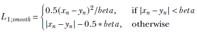
Equation 11.3
We can think of smooth L1 loss as a combination of L1 and L2 loss. If the value is < beta, it behaves like an L2 loss (mean squared error [MSE]). Otherwise, it behaves like an L1 loss. In the case of the FRCNN, beta is set to 1. The intuition behind this is simple. If we use pure L2 loss (MSE), then higher loss terms contribute to exponential loss because of the quadratic nature of the loss. This can lead to a bias where loss can be reduced by focusing on high-value items. Instead, if we use pure L1 loss, the higher loss terms still contribute more loss, but the effect is linear instead of quadratic. This still has a slightly worse bias toward higher loss terms. We get the best of both worlds by using L2 loss when the loss values are small and L1 loss when the loss values are large. When the loss value is small, because we are using L2 loss, its contribution is exponential/quadratic. And when the loss value is high, it still contributes linearly via L1 loss. Thus the network is incentivized to pay attention to low- and high-loss items.
Overall loss for an image can be defined as follows:
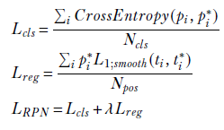
Equation 11.4
where, pi is the predicted objectness probability for the anchor i. pi* is the true objectness label for anchor i. It is 1 if the anchor is positive and 0 if the anchor is negative. ti = (tx, ty, tw, th) are the regression predictions for anchor i, ti* = (tx*, ty*, tw*, th*) are the regression targets for anchor i, Ncls is the number of anchors, and Npos is the number of positive anchors.
NOTE Fully functional code for the RPN loss function, executable via Jupyter Notebook, can be found at http://mng.bz/nY48.
Listing 11.20 PyTorch code for the RPN loss function
def rpn_loss(
    rpn_cls_scores, rpn_loc, rpn_labels,
    rpn_loc_targets, lambda_ = 10):                  ①


    classification_criterion = nn.CrossEntropyLoss(
        ignore_index=-1)                             ②
    reg_criterion = nn.SmoothL1Loss(reduction="sum")

    cls_loss = classification_criterion(rpn_cls_scores, rpn_labels)

    positive_indices = torch.where(rpn_labels==1)[0] ③
    pred_positive_anchor_offsets = rpn_loc[positive_indices]
    gt_positive_loc_targets = rpn_loc_targets[positive_indices]
    reg_loss = reg_criterion(
        pred_positive_anchor_offsets,
        gt_positive_loc_targets) / len(positive_indices)
    return {
        "rpn_cls_loss": cls_loss,
        "rpn_reg_loss": reg_loss,
        "rpn_total_loss": cls_loss + lambda_* reg_loss

    }
① rpn_cls_scores: (num_anchors, 2) tensor representing RPN classifier scores for each anchor. rpn_loc: (num_anchors, 4) tensor representing RPN regressor predictions for each anchor. rpn_labels: (num_anchors) representing the class for each anchor (-1, 0, 1). rpn_loc_targets: (num_anchors, 4) tensor representing RPN regressor targets for each anchor.
② Ignores -1 as they are not sampled
③ Finds the positive anchors
Generating region proposals
We have so far discussed how the RPN works. The RPN predicts objectness and the regression offsets for every anchor. The next task is to generate good region RoIs and use them for training the R-CNN module. Since we are emitting objectness and regression offsets for every anchor, we have thousands of predictions. We cannot use all of them as RoIs. We need to generate the best RoIs from these scores and offsets to train our R-CNN. An obvious way to do this is to rely on the objectness scores: the higher the objectness score, the greater the likelihood that it contains an object and thus is a good RoI. Before we get there, we must do some basic processing steps:
1. Convert the predicted offsets to bounding boxes. This is done by reversing the sequence of transformations
x∗ = tx∗ ∗ wa + xa
y∗ = ty∗ ∗ ha + ya
w∗ = etw∗ ∗ wa
h∗ = eth∗ ∗ ha
Equation 11.5
where x*, y*, w*, and h* denote the predicted bounding box’s center coordinates and its width and height, and tx*, ty*, tw*, and th* are the RPN loc predictions. The bounding boxes are then converted back into xtl, ytl, xbr, ybr format.
2. The predicted bounding boxes can lie partially outside the image. We clip all the predicted bounding boxes to within the image.
3. Remove any predicted bounding boxes with height or width less than min_roi_threshold.
Once these processing steps are done, we sort the predicted bounding boxes by objectness score and select N candidates. N = 12000 during training and N = 6000 while testing.
NOTE Fully functional generating region proposals from the RPN output, executable via Jupyter Notebook, can be found at http://mng.bz/nY48.
Listing 11.21 PyTorch code to generate region proposals from RPN output
rois = generate_bboxes_from_offset(rpn_loc, anchors)

rois = rois.clamp(min=0, max=width)       ①

roi_heights = rois[:, 3] - rois[:, 1]     ②
roi_widths = rois[:, 2] - rois[:, 0]
min_roi_threshold = 16

valid_idxes = torch.where((roi_heights > min_roi_threshold) &
    (roi_widths > min_roi_threshold))[0]
rois = rois[valid_idxes]
valid_cls_scores = rpn_loc[valid_idxes]


objectness_scores = valid_cls_scores[:, 1]

sorted_idx = torch.argsort(               ③
    objectness_scores, descending=True)
n_train_pre_nms = 12000
n_val_pre_nms = 300

rois = rois[sorted_idx][:n_train_pre_nms] ④

objectness_scores = objectness_scores[
    sorted_idx][:n_train_pre_nms]         ⑤
① Clips the ROIs
② Threshold based on min_roi_threshold
③ Sorts based on objectness
④ Selects the top regions of interest. Shape: (n_train_pre_nms, 4).
⑤ Selects the top objectness scores. Shape: (n_train_pre_nms,).
Non-maximal suppression (NMS)
Many of the proposals will overlap. We are effectively selecting anchors at a stride of 16 pixels. Therefore even a reasonably sized object is picked up by multiple anchors, each of which will try to predict the object independently. We can see this overlapping nature when we look at the positive anchors in figure 11.16. We want to choose the most effective set of RoIs. But it is evident that choosing all the similar proposals does not make a good set of RoIs because they carry redundant information.
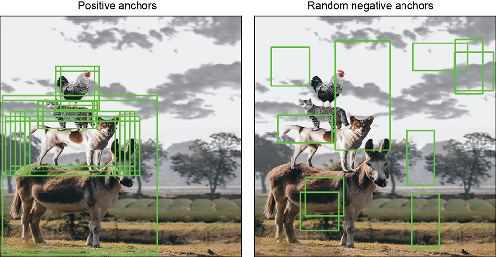
Figure 11.16 minimum where every anchor is classified as negative. To prevent this, the FRCNN under-samples the negative anchors before training.
To address this problem, we use a technique called non-maximal suppression (NMS). NMS is an algorithm that suppresses highly overlapping bounding boxes. The algorithm takes in bounding boxes and scores and works as follows.
Algorithm 11.6 Non-maximal suppression
Input: A list of bounding boxes B, corresponding scores S, and overlap threshold N
Output: A list of filtered bounding boxes D
while likelihood is increasing do
Select bounding box with highest confidence score
Remove it from B and add it to the final list D
Compare selected bounding box with remaining boxes in B using IoU
Remove all bounding boxes from B with IoU > threshold
end while
return D
We use NMS with a 0.7 threshold to suppress the highly overlapping RoIs and choose the top N RoIs post-NMS to train the R-CNN. N = 2000 during training, and N = 300 while testing. Figure 11.17 shows bounding boxes on a sample image before and after NMS.
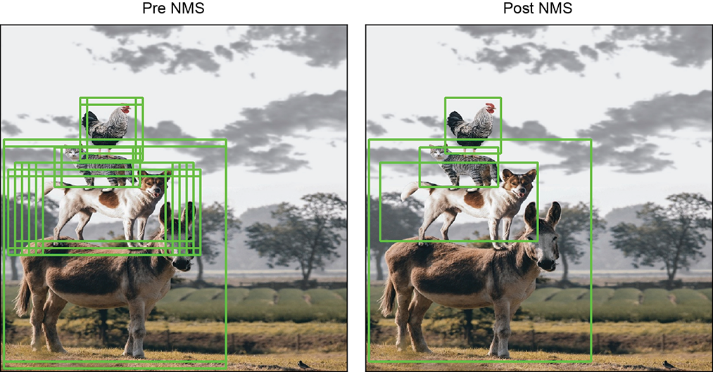
Figure 11.17 The left column shows the bounding boxes (24) before NMS. The right column shows the bounding boxes (4) that remain after NMS.
NOTE Fully functional code for NMS, executable via Jupyter Notebook, can be found at http://mng.bz/nY48.
Listing 11.22 PyTorch code for NMS of RoIs
n_train_post_nms = 2000
n_val_post_nms = 300
nms_threshold = 0.7

post_nms_indices = torchvision.ops.nms(     ①
    rois, objectness_scores, nms_threshold)


post_nms_rois = rois[post_nms_indices[:n_train_post_nms]]
① Calls NMS implemented by torchvision
11.4.3 Fast R-CNN
In the previous section, we saw how the RPN network takes an input image and emits a set of regions of interest that are likely to contain objects. Now let’s discuss the second leg of the FRCNN architecture, which takes in the RoIs and generates class probabilities and bounding-box coordinates for each object in the image. We briefly discussed this earlier. Here we revisit it in greater detail.
We are given a set of RoIs (some of which contain the object). Our task is to train an object detector capable of localizing the objects. To do this, we need to extract the features corresponding to each RoI and pass them through a neural network (classifier and regressor) that learns to predict the class and the regression targets. The R-CNN solved this in a naive way: it extracted each RoI one at a time, warped it to make it a fixed size, and passed it through a deep CNN to extract the features corresponding to the RoI. Each RoI required a separate forward pass, making the approach very slow. The question, as always, is: can we do better?
RoI pooling
Let’s consider the convolutional backbone. It processes the whole image with several conv and max pooling layers to produce a conv feature map. We have also seen a subsampling factor of 16: that is, 16 × 16 pixels in the input image are reduced to a single point in the feature map. Also remember that the embedding at every grid point on the feature map is the representation/digest of a region in the input image.
Key idea 1 is that the features corresponding to each RoI are already present in the conv feature map, and we can extract them via the feature map. For example, say our RoI is (0, 0, 256, 256). We know that the (0, 0, 256, 256) region in the input image is represented by 0, 0, 256/16, 256/16): that is, the (0, 0, 16, 16) region in the conv feature map. Since the embedding for a point in the conv feature map is a digest of the receptive field, we can use these features directly as the features of the RoI. So to obtain the features for an RoI of (0, 0, 256, 256), we take all the embeddings corresponding to the region (0, 0, 16, 16) in the conv feature map. Since we are performing this feature extraction directly on the convolutional feature map, which is obtained for the entire image, we can obtain the RoI features for all the RoIs in a single forward pass. This eliminates the need for multiple forward passes.
Key idea 2 is as follows. We discussed a clever way of extracting the features corresponding to each RoI, and we want to use these features to train our classifier and regressor. However, there is a problem. As we know, RoIs are different sizes. And different-sized RoIs will lead to different feature embedding sizes. For example, if our RoI is (0, 0, 256, 256), our RoI feature embeddings are (16, 16, 512): that is, all the embeddings (of size 512) in the (0, 0, 16, 16) region of the conv feature map. If our RoI is (0, 0, 128, 128), then our RoI feature embeddings are (8, 8, 512): all the embeddings in the (0, 0, 8, 8) region of the conv feature map. And we know that neural networks typically need same-sized input. So how do we deal with input embeddings of different sizes? The answer is RoI pooling.
Let’s fix the size of the input ROI feature map that goes into the neural network. Our task is to reduce variable-sized RoI feature maps to a fixed size. If the fixed feature map size is set to be H, W, and our RoI corresponds to (r, c, h, w) in the conv feature map, we divide h and w into equal-sized blocks of size h/H and w/W, respectively, and apply max pooling on these blocks to obtain a H, W feature map. Going back to our example, let’s fix H = W = 4. Our expected fixed feature map size is (4,4,512). So when our RoI is (0, 0, 256, 256), our RoI feature embeddings are (16, 16, 512): h = w = 16. We divide the 16 × 16 region into four 16/4, 16/4) regions and perform max pooling on each region to obtain a fixed-size (4,4,512) feature. Similarly, when our RoI is (0, 0, 128, 128), h = w = 8. We divide the 8 × 8 region into four (8/4, 8/4) regions and perform max pooling to obtain the fixed-size (4,4,512) feature.
Astute readers will notice that we have carefully chosen our RoIs so that they are multiples of H and W, resulting in integer values for h/H and w/W, respectively. But in reality, this rarely happens. h/H and w/W are often floating-point numbers. What do we do in this case? The answer is quantization: that is, we choose the integer closest to h/H and w/W, respectively (floor operation, in the original implementation). This has been improved on by RoIAlign, which uses bilinear interpolation instead of quantization. We do not get into the details of RoIAlign here.
In effect, if we have a large RoI, we divide the feature map into a fixed number of large regions and perform max pooling. And when we have a small RoI, we divide the feature map into a fixed number of small regions and perform max pooling. The size of the region used for pooling can change, but the output size remains fixed. The dimension of the RoI pooling output doesn’t depend on the size of the input feature map or the size of the RoIs: it’s determined solely by the number of sections we divide the RoI into—H and W (see figure 11.18).
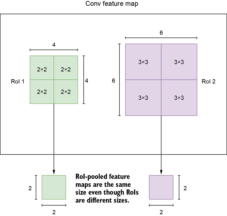
Figure 11.18 A conv feature map with two regions of interest of different sizes. RoI pooling extracts a fixed-sized output feature map (2 × 2 in this image) from each of the RoIs in a single pass via max pooling. This enables us to extract fixed-sized representative feature vectors for each RoI, which are then fed into further classifier and regressor layers for classification and localization.
Thus, the purpose of RoI pooling is to perform max pooling on inputs of non-uniform sizes to obtain fixed-size feature maps. The Fast R-CNN and Faster R-CNN use 7 × 7 as the fixed feature map size.
Fast R-CNN architecture
Given the conv feature map and a set of RoIs, we have seen how the RoI pooling layer extracts a fixed-length feature vector from the feature map. Each feature vector is fed into a sequence of FC layers that finally branch into two sibling output layers: a classifier that produces softmax probability estimates over K object classes plus a catch-all “background” class, and a regressor that produces four real-valued numbers for each of the K object classes.
Generating GT for the Fast R-CNN
For every image, we have a list of RoIs generated by the RPN and a list of GT bounding boxes. How do we generate the GT and regression targets for each RoI? The idea remains the same as for our RPN: we use IoU scores. The algorithm is as follows:
-
Compute the IoU between all RoIs and GT boxes.
-
For each RoI, determine the GT bounding box with the highest IoU.
-
If the highest IoU is greater than a threshold (0.5), assign the corresponding GT label as the label for the RoI.
-
If the IoU is between [0.1, 0.5], assign the background label. Using a lower bound of 0.1 ensures that certain RoIs with small intersections with the GT are selected as background. This is helpful as it chooses hard examples for background; it is a form of hard negative mining.
NOTE Fully functional code for the Fast R-CNN RoI head, executable via Jupyter Notebook, can be found at http://mng.bz/nY48.
Listing 11.23 PyTorch code for the Fast R-CNN RoI head
class Fast_RCNN_ROI_Head(nn.Module):
    def __init__(self, num_classes, H, W, subsample=16, embedding_size=512):

        super(Fast_RCNN_ROI_Head, self).__init__()

        self.num_classes = num_classes
        self.H = H
        self.W = W
        self.embedding_size = embedding_size
        self.subsample = 16

        self.roi_head_classifier = nn.Sequential(
            nn.Linear(H*W*embedding_size, 4096),
            nn.ReLU(True),
            nn.Linear(4096, 4096),
            nn.ReLU(True),
        )
        self.cls = torch.nn.Linear(4096, num_classes+1) ①
        self.reg = torch.nn.Linear(4096, (num_classes+1)*4)

    def forward(self, x, rois):                         ②
        assert x.shape[0] == 1 # This code only supports batch size of 1
        roi_pooled_features = torchvision.ops.roi_pool(
            x, [rois], output_size=(self.H, self.W), spatial_scale=1/subsample)
        roi_pooled_features = roi_pooled_features.view(
            -1, self.H*self.W*self.embedding_size)
        fc_out = self.roi_head_classifier(roi_pooled_features)
        roi_cls_scores = self.cls(fc_out)
        roi_loc = self.reg(fc_out)

        return roi_cls_scores, roi_loc                  ③
① num_classes + background
② x : (1, c, h, w) tensor representing the conv feature map. rois: (n, 4) tensor representing bounding boxes of RoIs
③ roi_cls_scores: (n, num_classes+1) tensor representing classification scores for each RoI. roi_loc: (n, (num_classes + 1) * 4) tensor representing the regression scores for each RoI
Training the Fast R-CNN
The RPN generates about 2,000 RoIs per image. Due to computational constraints, we cannot use all N RoIs. Instead, we sample a subset of them. The training minibatches are sampled hierarchically, first by sampling K images and then by sampling R/K RoIs from each image. R is set to 128 in the FRCNN. For this discussion, we assume that K = 1: that is, we have a single image per minibatch. So, given the RoIs for a single image, how do we sample 128 RoIs from it?
A simple solution is to randomly sample 128 RoIs. However, this runs into the same data-imbalance issue that we discussed earlier: we end up sampling backgrounds a lot more frequently than the classes. To solve this problem, we adopt a sampling strategy similar to before. In particular, for a single image, we sample 128 RoIs such that the ratio of background to object is 0.75:0.25. If fewer than 32 RoIs contain the objects, we pad the minibatch with more background RoIs.
Assigning targets to RoI boxes
Just as in the case of the RPN, we generate regression targets as offsets of the GT box from the region of interest for all RoIs that contain objects. For all background RoIs, the regression targets are not applicable.
Fast R-CNN loss function
We have defined the Fast R-CNN network and how we can generate labels and regression targets for its outputs. We need to discuss the loss function that enables us to train the Fast R-CNN. As you would expect, there are two loss terms:
-
Classification loss— We use the standard cross-entropy loss used in any standard classifier.
-
Regression loss—The regression loss applies only to the object RoIs: background RoIs do not contribute to regression. Here we use the smooth L1 loss as we did in the RPN.
Thus the overall loss for a single RoI can be defined as follows:
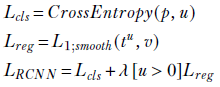
Equation 11.6
where p is the predicted label for the RoI, u is the true label for the RoI, tu = (tx, ty, tw, th) are the regression predictions for class u, and v = (vx, vy, vw, vh) are the regression targets. The overall loss can therefore be defined as
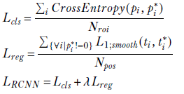
Equation 11.7
where pi are the prediction probabilities for the RoI i, pi* is the true label for RoI i; ti = (tx, ty, tw, th) are the regression predictions for RoI i corresponding to class pi*, ti* = (tx*, ty*, tw*, th*) are the regression targets for RoI i, ti* = (tx*, ty*, tw*, th*) are the regression targets for RoI i, and Npos is the number of object RoIs (non-background RoIs).
NOTE Fully functional code for the Fast R-CNN loss function, executable via Jupyter Notebook, can be found at http://mng.bz/nY48.
Listing 11.24 PyTorch code for the Fast R-CNN loss function
def rcnn_loss(
    roi_cls_scores,                              ①
    roi_loc,                                     ②
    roi_labels,                                  ③
    rcnn_loc_targets,                            ④
    lambda_ = 1):

    classification_criterion = nn.CrossEntropyLoss()
    reg_criterion = nn.SmoothL1Loss(reduction="sum")

    cls_loss = classification_criterion(roi_cls_scores, roi_labels)

    pos_roi_idxes = torch.where(roi_labels>0)[0] ⑤
    pred_all_offsets = roi_loc[pos_roi_idxes]

    num_pos_rois = len(pos_roi_idxes)
    pred_all_offsets = pred_all_offsets.view(    ⑥
        num_pos_rois, -1, 4)

    pred_cls_offsets = pred_all_offsets[
        torch.arange(num_pos_rois) , roi_labels[pos_roi_idxes]]

    gt_offsets = rcnn_loc_targets[pos_roi_idxes]

    reg_loss = reg_criterion(pred_cls_offsets, gt_offsets) / num_pos_rois
    return {
        "rcnn_cls_loss": cls_loss,
        "rcnn_reg_loss": reg_loss,
        "rcnn_total_loss": cls_loss + lambda_* reg_loss

    }
① (128, num_classes) tensor: RCNN classifier scores for each RoI
② (128, num_classes*4) tensor: RCNN regressor predictions for each class, RoI
③ (128,) tensor: true class for each RoI
④ (128, 4) tensor: RoI regressor targets for each RoI
⑤ Finds the positive RoIs
⑥ (n, num_classes*4) to n, num_classes, 4)
Fast R-CNN inference
We have looked at how to train the Fast R-CNN module. Once the model is trained, the next question is how to use the model to generate output classes and bounding boxes.
The Fast R-CNN model outputs a classification score and regression offsets for every RoI. We can safely ignore the background RoIs. For the rest of the RoIs, the class with the highest probability is chosen as the output label, and the offsets corresponding to that class are chosen. We apply post-processing steps similar to that of the RPN:
-
We translate the offsets back to (
xtl,ytl,xbr,ybr) format using the RoI. -
We clip the output bounding box to within the image boundaries
We face a problem similar to before: the output probably has multiple bounding boxes corresponding to the same object. We deal with it in the same way as earlier: using NMS. There is one difference, however. In the case of the RPN, we applied a global NMS across all bounding boxes predicted by the RPN. Here, NMS is applied only across the bounding boxes belonging to the same class. This is done for all classes, which should intuitively make sense: there is no point in suppressing highly overlapping bounding boxes if the bounding boxes represent different classes.
NOTE Fully functional code for the Fast R-CNN inference, executable via Jupyter Notebook, can be found at http://mng.bz/nY48.
Listing 11.25 PyTorch code for the Fast R-CNN inference
def fast_rcnn_inference(
    frcnn_roi_head,                                      ①
    rois,                                                ②
    conv_feature_map,                                    ③
    nms_threshold=0.7):

    frcnn_roi_head.eval()                                ④
    roi_cls_scores, roi_loc = frcnn_roi_head(conv_feature_map, rois)

    output_labels = torch.argmax(                        ⑤
        roi_cls_scores, dim=1)

    output_probs = nn.functional.softmax(
        roi_cls_scores, dim=1)[torch.arange(             ⑥
            rois.shape[0]), output_labels]

    output_offsets = roi_loc.view(                       ⑦
        rois.shape[0], -1, 4)


    output_offsets = output_offsets[                     ⑧
        torch.arange(rois.shape[0]), output_labels]


    assert output_offsets.shape == torch.Size(           ⑨
        [rois.shape[0], 4])

    output_bboxes = generate_bboxes_from_offset(         ⑩
        output_offsets, rois)

    rois = output_bboxes.clamp(min=0, max=width)         ⑪

    post_nms_labels, post_nms_probs, post_nms_boxes = [], [], []

    for cls in range(1, frcnn_roi_head.num_classes+1):   ⑫

        cls_idxes = torch.where(output_labels == cls)[0] ⑬
        cls_labels = output_labels[cls_idxes]
        cls_bboxes = output_bboxes[cls_idxes]
        cls_probs = output_probs[cls_idxes]
        keep_indices = torchvision.ops.nms(
            cls_bboxes, cls_probs, nms_threshold)

        post_nms_labels.append(cls_labels[keep_indices])
        post_nms_probs.append(cls_probs[keep_indices])
        post_nms_boxes.append(cls_bboxes[keep_indices])

    return {
        "labels": torch.cat(post_nms_labels),
        "probs": torch.cat(post_nms_probs),
        "bboxes": torch.cat(post_nms_boxes)
    }
① Trained instance of Fast_RCNN_ROI_Head
② RoIs to inference
③ (n, c, h, w) convolutional feature map
④ Sets eval mode
⑤ The predicted class is the class with the highest score.
⑥ The predicted probabilities are obtained via softmax. The highest probability is chosen as the probability score for this prediction.
⑦ Converts locs from (n, num_classes*4) to (n, num_classes, 4)
⑧ Selects offsets corresponding to the predicted label
⑨ Asserts that we have outputs for each RoI
⑩ Converts offsets to xtl, ytl, xbr, ybr)
⑪ Clips bounding boxes to within images
⑫ 0 is background, thus ignored
⑬ Performs NMS for each class
11.4.4 Training the Faster R-CNN
As we have seen, the FRCNN consists of two subnetworks:
-
An RPN responsible for generating good region proposals that contain objects
-
A Fast R-CNN responsible for object classification and detection from a list of RoIs
Thus the FRCNN is a two-stage object detector. We have one stage that generates good region proposals and another that takes the region proposals and detects objects in the image. So how do we train the FRCNN?
A simple idea would be to train two independent networks (RPN and Fast R-CNN). However, we do not want to do this because it is expensive. Additionally, if we do so, each network will modify the convolutional layers in its own way. As discussed earlier, we want to share the convolutional layers across the RPN and the Fast R-CNN modules. This ensures efficiency (only one conv backbone as opposed to two independent backbones). Additionally, both the RPN and FRCNN are performing similar tasks, so it intuitively makes sense to share the same set of convolutional features. Therefore, we need to develop a technique that allows for sharing convolutional layers between the two networks rather than learning two separate networks. The original FRCNN paper proposed two techniques to train the model:
-
Alternate optimization (AltOpt)—We first train RPN and use the proposals to train the Fast R-CNN. The network tuned by the Fast R-CNN is then used to initialize the RPN, and this process is iterated. This involves multiple rounds of training alternating between training the RPN and Fast R-CNN.
-
Approximate joint training—The RPN and Fast R-CNN networks are merged into one network during training. In each SGD iteration, the forward pass generates region proposals that are treated just like fixed, precomputed proposals when training a Fast R-CNN detector. We combine the RPN and Fast R-CNN losses and perform backpropagation as usual. This training is significantly faster as we are training both networks together end to end. However, the optimization is approximate because we treat the RPN-generated proposals as fixed, whereas in reality, they are a function of the RPN. So, we’re ignoring one derivative.
Both techniques give similar accuracy. So joint training, which is significantly faster, is preferred.
11.4.5 Other object-detection paradigms
So far, we have looked at the FRCNN in detail and discussed several key ideas that contribute to its success. Several other object-detection paradigms have also been developed. Some are inspired by the FRCNN, borrowing and/or improving on the ideas established by the FRCNN. In this section, we briefly look at a few of them.
You Only Look Once (YOLO)
The FRCNN is a two-stage detector: an RPN followed by the Fast R-CNN, which runs on the region proposals generated by the RPN. YOLO (https://arxiv.org/pdf/1506.02640.pdf), as the name implies, is a single-stage object detector. A single convolutional network simultaneously predicts multiple bounding boxes and class probabilities for those boxes directly from full images in one go. Some of the salient features of YOLO are as follows:
-
YOLO is significantly faster ( 10× faster than the FRCNN) due to its much simpler architecture. YOLO can even be used for real-time object detection.
-
Unlike the FRCNN, where the R-CNN module looks only at the region proposals, YOLO looks directly at the full image during training and testing.
-
The speed of YOLO comes at the cost of accuracy. While YOLO is significantly faster, it is less accurate than the FRCNN.
Several other improvements have been made on top of YOLO to improve accuracy while trying to maintain the simple, fast architecture. These include YOLO v2, YOLO v3, and so on.
MultiBox Single-Shot Detector SSD)
SSD (https://arxiv.org/pdf/1512.02325.pdf) tries to achieve a good balance between speed and accuracy. It is a single-stage network like YOLO: that is, it eliminates the proposal-generation (RPN) and subsequent feature-resampling stages. It also borrows the ideas of anchors from the FRCNN: applying a conv net on top of feature maps to make predictions relative to a fixed set of bounding boxes.
Thus, a single deep network predicts class scores and box offsets for a fixed set of default bounding boxes using small convolutional filters applied to feature maps. To achieve high detection accuracy, feature maps at different scales are used to make predictions at different scales.
SSD is much more accurate than YOLO; however, it is still not as accurate as the FRCNN (especially for small objects).
Feature pyramid network (FPN)
The feature maps generated by conv nets are pyramidal: as we go deeper, the spatial resolution of the feature map keeps decreasing, and we expect the semantic information represented by the feature map to be more meaningful. High-resolution maps have low-level features, whereas low-resolution maps have more semantic features.
In the case of the FRCNN, we applied object detection on only the last convolution map. SSD shows that there is useful information by using other feature maps for prediction. But SSD builds this pyramid high up the network (past the fourth convolution layer [conv4] of VGG). It specifically avoids the use of lower-layer features. Thus it misses the opportunity to reuse the higher-resolution maps of the feature hierarchy. FPN shows that these features are important, especially for detecting small objects.
The FPN (https://arxiv.org/pdf/1612.03144.pdf) relies on an architecture that combines low-resolution, semantically strong features with high-resolution, semantically weak features via a top-down pathway and lateral connections. The bottom-up pathway is the forward pass of the convolutional layers. In the top-down path, there is a back connection from lower resolution to higher resolution via simple upsampling (it is merged with the bottom-up feature map using 1 × 1 convolutions). This merged feature map is used at every level to learn and make predictions.
The FPN was originally implemented on top of the FRCNN. It is much more accurate, but it is much slower than YOLO/SSD-style approaches.
We have only briefly mentioned the other prominent detection paradigms. The fundamental principles behind them remain the same. You are encouraged to read the papers to get a deeper and better understanding.
Summary
In this chapter, we took an in-depth look at various deep-learning techniques for object classification and localization:
-
LeNet is a simple neural network that can classify handwritten digits from the MNIST data set.
-
Simple networks like LeNet don’t extend well to more real-world image classification problems. Hence deeper neural networks that have more expressive power are needed.
-
The VGG network is one of the most popular deep convolutional neural networks. It improves on prior state-of-the-art deep neural networks by using more convolution layers with smaller 3 × 3) filters. Such an architecture has two advantages: (1) more expressive power because of the added nonlinearity that comes from stacking more layers, and (2) a reduced number of parameters. Three 3 × 3 filters have 27C2 parameters, whereas a single 7 × 7 filter (which cover the same receptive field) has 49C2 parameters (81% more).
-
VGG (and AlexNet) use ReLU nonlinear layers instead of sigmoid layers because they do not suffer from the vanishing gradient problem. Using ReLUs speeds up training, resulting in faster convergence.
-
Inception blocks provide an efficient way to increase the depth and width of a neural network while keeping the computational budget constant. Multiscale filters are used at each convolution layer to learn patterns of different sizes, and 1 × 1 convolutions are used for dimensionality reduction (which reduces the number of parameters needed, thereby improving computational efficiency).
-
ResNet is another popular convolutional neural network. The ResNet architecture was motivated by the fact that simply stacking layers beyond a certain point does not help and causes degradation even in training accuracies. This is a counterintuitive result because we expect that deeper networks can, at the very least, learn as much as their shallower counterparts. The authors of the ResNet papers showed that this may happen because the identity function is hard for neural networks to learn. To tackle this, they proposed shortcut/skip connections to simplify the neural network’s learning objective. This is the key idea behind ResNet and enables training of much deeper neural networks.
-
Faster R-CNN is one of the most popular object detectors. It is a two-stage network consisting of (1) a region proposal network RPN), which is responsible for predicting regions of interest that could potentially contain objects; and (2) an R-CNN module, which takes the region proposals as input and emits class scores and bounding boxes efficiently.
-
The RPN module uses multiple anchor boxes (at each point on the conv feature map) to handle objects of different sizes and aspect ratios. It convolves a small network over the conv feature map to make predictions about objectness and bounding boxes at each sliding window location. Remember that the small network is a fully convolutional network (FCN) comprising 3 × 3 convs followed by 1 × 1 convs, enabling this approach to work with arbitrary-sized inputs and making it translation invariant.
-
RoI pooling provides an efficient way to extract a fixed-sized feature vector from region proposals of varying sizes, all in one pass. These feature vectors are fed to a classifier and regressor for classification and localization, respectively.
-
Non-maxima suppression (NMS) is a technique to de-duplicate overlapping bounding boxes.
-
FRCNN can be trained using two methods: alternative optimization (AltOpt) and approximate joint training. Both approaches lead to similar accuracy numbers, but approximate joint training is significantly faster.
-
You Only Look Once (YOLO), MultiBox Single-Shot Detector SSD), and feature pyramid networks (FPN) are some other popular object detectors.