13 Fully Bayes model parameter estimation
This chapter covers
- Fully Bayes parameter estimation for unsupervised modeling
- Injecting prior belief into parameter estimation
- Estimating Gaussian likelihood parameters with known or unknown mean and precision
- Normal-gamma and Wishart distributions
Suppose we have a data set of interest: say, all images containing a cat. If we represent images as points in a high-dimensional feature space, our data set of interest forms a subspace of that feature space. Now we want to create an unsupervised model for our data set of interest. This means we want to identify a probability density function p(![]() ) whose sample cloud (the set of points obtained by repeatedly sampling the probability distribution many times) largely overlaps our subspace of interest. Of course, we do not know the exact subspace of interest, but we have collected a set of samples X from the data set of interest: that is, the training data. We can use the point cloud for X as a surrogate for the unknown subspace of interest. Thus, we are essentially trying to identify a probability density function p(
) whose sample cloud (the set of points obtained by repeatedly sampling the probability distribution many times) largely overlaps our subspace of interest. Of course, we do not know the exact subspace of interest, but we have collected a set of samples X from the data set of interest: that is, the training data. We can use the point cloud for X as a surrogate for the unknown subspace of interest. Thus, we are essentially trying to identify a probability density function p(![]() ) whose sample cloud, by and large, overlaps X.
) whose sample cloud, by and large, overlaps X.
Once we have the model p(![]() ), we can use it to generate more data samples; these will be computer-generated cat images. This is generative modeling. Also, given a new image
), we can use it to generate more data samples; these will be computer-generated cat images. This is generative modeling. Also, given a new image ![]() , we can estimate the probability of it being an image of a cat by evaluating p(
, we can estimate the probability of it being an image of a cat by evaluating p(![]() ).
).
13.1 Fully Bayes estimation: An informal introduction
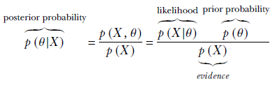
Equation 13.1
Here, X = {![]() 1,
1, ![]() 2,⋯} denotes the training data set. Our ultimate goal is to identify the likelihood function p(
2,⋯} denotes the training data set. Our ultimate goal is to identify the likelihood function p(![]() |θ). Estimating the likelihood function has two aspects: selecting the function family and estimating the parameters. We usually preselect the family from our knowledge of the problem and then estimate the model parameters. For instance, the family for our model likelihood function might be Gaussian: p(
|θ). Estimating the likelihood function has two aspects: selecting the function family and estimating the parameters. We usually preselect the family from our knowledge of the problem and then estimate the model parameters. For instance, the family for our model likelihood function might be Gaussian: p(![]() |θ) = 𝒩(
|θ) = 𝒩(![]() ;
; ![]() , Σ) as before, the semicolon separates the model variables from model parameters). Then θ = {
, Σ) as before, the semicolon separates the model variables from model parameters). Then θ = {![]() , Σ} are the model parameters to estimate. We estimate θ such that the overall likelihood p(X|θ) = ∏i p(
, Σ} are the model parameters to estimate. We estimate θ such that the overall likelihood p(X|θ) = ∏i p(![]() i|θ) best fits the training data X.
i|θ) best fits the training data X.
We want to re-emphasize the mental picture that best fit implies that the sample cloud of the likelihood function (repeated samples from p(![]() |θ)) largely overlaps the training data set X. For the Gaussian case, this implies that the mean
|θ)) largely overlaps the training data set X. For the Gaussian case, this implies that the mean ![]() should fall at a place where there is a very high concentration of training data points, and the covariance matrix Σ should be such that the elliptical base of the likelihood function tightly contains as many training data points as possible.
should fall at a place where there is a very high concentration of training data points, and the covariance matrix Σ should be such that the elliptical base of the likelihood function tightly contains as many training data points as possible.
13.1.1 Parameter estimation and belief injection
There are various possible approaches to parameter estimation. The simplest approach is maximum likelihood parameter estimation MLE), introduced in section 6.6.2. In MLE, we choose the parameter values that maximize p(X|θ), the likelihood of observing the training data set. This makes some sense. After all, the only thing we know to be true is that the input data set X has been observed—this being unsupervised data, we do not know anything else. It is reasonable to choose the parameters that maximize the probability of that known truth. If the training data set is large, MLE estimation works well.
However, in the absence of a sufficiently large amount of training data, it often helps to inject our prior knowledge about the system into the estimation—prior knowledge can cover for the lack of data. This injection of guess/belief into the system is done via the prior probability density. To do this, we can no longer maximize the likelihood, as likelihood ignores the prior. We have to do maximum a posteriori (MAP) estimation, which maximizes the posterior probability. The posterior probability is the product of likelihood (which depends on the data) and the prior (which does not depend on data; we will make it reflect our prior belief).
There are two possible MAP paradigms. We saw one of them in section 6.6.3, where we injected our belief that the unknown parameters must be small in magnitude and set p(θ) ∝ e−||θ||2 as a regularizer. The system was incentivized to select parameter values that are relatively smaller in magnitude. In this chapter, we study a different paradigm; let’s illustrate it with an example.
Suppose we model the likelihood as a Gaussian: p(![]() |θ) = 𝒩(
|θ) = 𝒩(![]() ;
; ![]() , Σ). We have to estimate the parameters θ = {
, Σ). We have to estimate the parameters θ = {![]() , Σ} from the training data X, for which we must maximize the posterior probability. To compute the posterior probability, we need the prior probability. In addition, we must somehow inject constant values as our belief (lacking observed data) about the parameter values. How about modeling the prior probability as a Gaussian probability density function in the parameter space? Ignoring the covariance matrix parameter for the sake of simplicity, we can model the probability density of the mean parameter as p(
, Σ} from the training data X, for which we must maximize the posterior probability. To compute the posterior probability, we need the prior probability. In addition, we must somehow inject constant values as our belief (lacking observed data) about the parameter values. How about modeling the prior probability as a Gaussian probability density function in the parameter space? Ignoring the covariance matrix parameter for the sake of simplicity, we can model the probability density of the mean parameter as p(![]() ) = 𝒩(
) = 𝒩(![]() ;
; ![]() 0, Σ0). We are essentially saying that we believe the parameter
0, Σ0). We are essentially saying that we believe the parameter ![]() is likely to have a value near
is likely to have a value near ![]() 0 with a confidence Σ0. In other words, we are injecting a constant value as our belief in the parameter
0 with a confidence Σ0. In other words, we are injecting a constant value as our belief in the parameter ![]() . We can treat the covariance similarly. Later, we prove that in this paradigm, with a low volume of training data, the prior dominates. Once sufficient training data is digested, the effect of the prior fades, and the solution gets closer and closer to the MLE. This is the fully Bayes parameter estimation technique in a nutshell.
. We can treat the covariance similarly. Later, we prove that in this paradigm, with a low volume of training data, the prior dominates. Once sufficient training data is digested, the effect of the prior fades, and the solution gets closer and closer to the MLE. This is the fully Bayes parameter estimation technique in a nutshell.
In this chapter, we discuss Bayes estimation of parameters for a Gaussian likelihood function for a series of increasingly complex scenarios. In section 13.3, we deal with the case where the variance of the parameters to be estimated is known (constant) but the mean is unknown, so the mean is expressed as a (Gaussian) random variable. Then, in section 13.6, we examine the case where the mean is known (constant) but the variance is unknown. Finally, in section 13.7, we examine the case where both are unknown. Both the univariate and multivariate cases are dealt with for each scenario.
NOTE Fully functional code for this chapter, executable via Jupyter Notebook, can be found at http://mng.bz/woYW.
13.2 MLE for Gaussian parameter values recap)
We have discussed the details of this in section 6.8. Here we recap the main results. Suppose we have a data set X = {x(1), x(2),⋯, x(n)}. We have decided to model the data distribution as a Gaussian 𝒩(x;μ, σ)—we want to estimate the parameters μ, σ that best “explain" or “fit" the observed data set X. MLE is one of the simplest approaches to solving this problem. Here we estimate the parameters such that the likelihood of the data observed during training is maximized. This can be loosely visualized as estimating a probability density function whose peak coincides with the region in the input space with the densest population of training data. We looked at MLE in section 6.8. Here we simply restate the expressions.
Let’s denote the (as yet unknown) mean and variance of the data distribution as μ and σ. Then from equation 5.22, we get
Maximizing the log-likelihood p(X|μ, σ) has a closed-form solution:
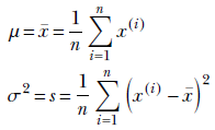
Equation 13.2
Thus the MLE mean and variance are essentially the mean and variance of the training data samples (see section 6.6 for the derivation of these expressions).
The corresponding expressions for multivariate Gaussian MLE are
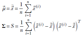
Equation 13.3
These MLE parameter values are to be used to evaluate p(x) = 𝒩(x;μ, σ)—the probability of an unknown data point x coming from the distribution represented by the training data set X.
13.3 Fully Bayes parameter estimation: Gaussian, unknown mean, known precision
MLE may not be that accurate when the available data set is small that is, n, size of the data set X, is small). In many problems, we have a prior idea of the mean and sigma of the data set. Unfortunately, MLE provides no way to bake such a prior belief into the estimation. Fully Bayes parameter estimation techniques try to fix this drawback: here we are not simply maximizing the likelihood of the observed data. Instead, we maximize the posterior probability of the estimated parameter(s). This posterior probability involves the product of the likelihood and a prior probability (see equation 13.1). The likelihood term captures the effect of the training data—maximizing it alone is MLE—but does not capture the effect of a prior belief. On the other hand, the prior term does not depend on the data. This is where we bake in our belief or guess or prior knowledge about the data distribution. Thus, our estimate for the data distribution parameters will consider the data and the prior guess. We will soon see that the estimation is such that as the size of the data set (n, length of X) increases, the effect of the prior term decreases, and the effect of the likelihood term increases. In the limit, at infinite data availability, the Bayesian inference ields the MLE. At the other extreme, when no data is available (n = 0), the Fully Bayes estimates for the parameters are the same as the prior estimates.
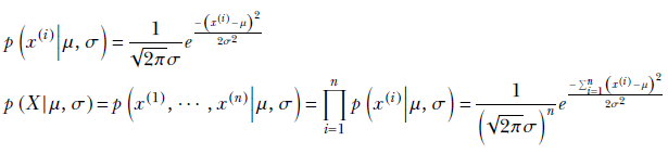
Let’s we examine Bayesian parameter estimation. For starters, we deal with a relatively simple case where we have a Gaussian data distribution with a known (constant) variance but unknown and modeled mean. The data distribution is Gaussian (as usual, the semicolon in 𝒩(x;μn, σ) separates the variables from parameters):
![]()
The training data set is denoted X = {x(1), x(2),⋯, x(n)}, and its overall likelihood is
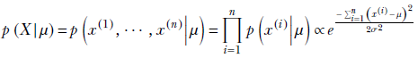
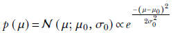
The variance is known by assumption—hence it is treated as a constant instead of a random variable. The mean μ is unknown and is treated as a Gaussian random variable, with mean μ0 and variance σ0 (not to be confused with μ and σ, the mean and variance of the data itself ). So, the prior is
The posterior probability of the unknown μ parameter is a product of two Gaussians, which is a Gaussian itself. Let’s denote the as-yet-unknown) mean and variance of this product Gaussian as μn and σn. Here the subscript n is to remind us that the posterior has been obtained by digesting n data instances from X = {x(1), x(2),⋯, x(n)}. Thus, the Gaussian posterior can be denoted as
![]()
Using Bayes’ theorem,
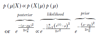
By comparing the coefficients of μ2 and μ on the exponents of the left and right sides, we determine the unknown parameters of the posterior distribution:
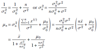
Equation 13.4
The significance of various closely named variables should be clearly understood:
-
μ, σ are the mean and variance of the data distribution p(x)—assumed to be Gaussian. The final goal is to estimate μ, σ that best fits the data set X. On the other hand, μ0, σ0 are the mean and variance of the parameter distribution p(μ), which captures our prior belief about the value of the data mean μ (remember, by assumption, the data mean is also a Gaussian random variable). μn, σn are the mean and variance of the posterior distribution p(μ|X) for the data mean μ as computed from n data point samples. This is a Gaussian random variable because it is a product of two Gaussians.
-
The posterior distribution of the unknown mean parameter, p(μ|X), is a Gaussian with mean μn. So, it will attain a maximum when μ = μn. In other words, the MAP estimate for the unknown mean μ is μMAP = μn.
-
Even though μn is the best estimate of μ, σn is not approximating the σ of the data, σ is known in this case by assumption. Here, σn is the variance of the posterior distribution, reflecting our uncertainty about the estimate of μ. That is why, as the number of data instances becomes very large, σn approaches 0 (indicating we have zero uncertainty or full confidence in the estimate of the mean.)
The estimate for our data distribution is p(x) = 𝒩(x;μn, σ), where μn is given by equation 13.4. Note that it is a combination of the MLE x̄ and prior guess μ0. Using this, given any arbitrary data instance x, we can infer the probability of x belonging to the class of the training data set X.
NOTE Fully functional code for Bayesian estimation with unknown mean and known variance, executable via Jupyter Notebook, can be found at http://mng.bz /ZA75.
Listing 13.1 PyTorch- Bayesian estimation with unknown mean, known variance
import torch

def inference_unknown_mean(X, prior_dist, sigma_known):
    mu_mle = X.mean()
    n = X.shape[0]

    mu_0 = prior_dist.mean
    sigma_0 = prior_dist.scale                             ①


    mu_n = mu_mle / (1 + sigma_known**2 / (n * sigma_0**2)) +
             mu_0 / (1 + n * sigma_0**2 / sigma_known**2)  ②

    sigma_n = math.sqrt(
        (sigma_0**2 * sigma_known**2) /
        (n*sigma_0**2+sigma_known**2))                     ③

    posterior_dist = torch.Normal(mu_n, sigma_n)
    return posterior_dist
① Parameters of the prior
② Mean of the posterior, following equation 13.4
③ Standard deviation of the posterior, following equation 13.4
13.4 Small and large volumes of training data, and strong and weak priors
Let’s examine the behavior of equation 13.4 when n = 0 (no data) and when n → ∞ (lots of data):
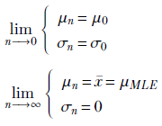
This agrees with our notion that with little data, the posterior is dominated by the prior, while with lots of data, the posterior is dominated by the likelihood. With lots of data, the variance of the parameter is zero (we are saying with full certainty that the best value for the mean is the sample mean for the data, aka the MLE estimate for the mean). In general, with more training data (that is, larger values of n), the posterior shifts closer to the likelihood. This can be seen by analyzing equation 13.4. It agrees with our intuition that with little data, we try to compensate with our pre-existing (prior) belief as to the value of the parameters. As the number of training data instances increases, the effect of the prior is reduced, and the likelihood (which is a function of the data) begins to dominate.
A low variance for the prior (that is, small σ0) essentially means we have low uncertainty in our prior belief (remember, the entropy/uncertainty of a Gaussian is proportional to its variance). Such high-confidence priors resist being overwhelmed by the data and are called strong priors. On the other hand, a large σ0 implies low /confidence in the prior mean value. This is a weak prior that is easily overwhelmed by the data. We can see this in the final expression for mean in equation 13.4: we have nσ02/σ2 in the denominator of the second term. In general, the second term vanishes with larger n, thereby removing the effect of the prior μ0 and making the posterior mean coincide with the MLE mean. But the smaller the σ0, the larger the n required to achieve this, and vice versa.
13.5 Conjugate priors
In section 13.3, given a Gaussian likelihood, choosing the Gaussian family for the prior made the posterior also belong to the Gaussian family. This simplified things considerably. If the prior was chosen from another family, the posterior—which is the product of the likelihood and prior—may not belong to a simple or even known distribution family.
Thus, a Gaussian likelihood with a Gaussian prior results in a Gaussian posterior for the mean. Such priors are said to be conjugate. Formally, for a specific family of likelihood, the choice of the prior that results in the posterior belonging to the same family as the prior is called a conjugate prior. For instance, Gaussians for the mean (with known variance) are conjugate to a Gaussian likelihood. Soon we will see that for a Gaussian likelihood, a gamma distribution for the precision (inverse of the variance) results in a gamma posterior. In other words, a gamma prior to the precision is conjugate to a Gaussian likelihood. In the multivariate case, instead of gamma, we have the Wishart distribution as a conjugate prior.
13.6 Fully Bayes parameter estimation: Gaussian, unknown precision, known mean
In section 13.3, we discussed fully Bayes parameter estimation with the assumption that we somehow know the variance σ and only want to estimate the mean μ. Now we examine the case where the mean is known but the variance is unknown and expressed as a random variable. The computations become simpler if we use precision λ instead of variance σ. They are related by the expression 1/σ2. Thus we have a data set X, which is assumed to be sampled from a Gaussian distribution with a constant mean μ, while the precision λ is a random variable with a gamma distribution. The probability density function for the data is thus p(x|μ, λ) = 𝒩(x; μ, 1/√λ).
We model the prior random variable for precision with a gamma distribution. The likelihood is Gaussian, and since the product of a Gaussian and gamma is another gamma (due to the conjugate prior property of gamma), the resulting posterior is a gamma. The gamma function parameters for the posterior can be derived via coefficient comparison. The maximum of the posterior is our estimate for the parameter.
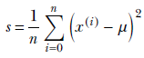
13.6.1 Estimating the precision parameter
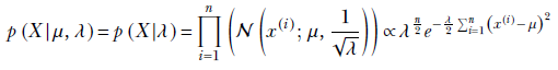
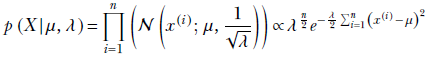
Let’s return to the fully Bayes estimation of the precision parameter when the mean is known. We model the data distribution with a Gaussian: p(x|μ, λ) = 𝒩(x; μ, 1/√λ) (we have expressed this Gaussian in terms of the precision, λ, which is related to the variance σ as λ = 1/σ 2). The training data set is X = {x(1), x(2),⋯, x(n)}, and its overall likelihood is
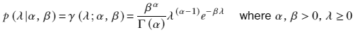
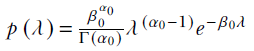
We model the prior for the precision with a gamma distribution with parameters α0, β0:
p(λ) = γ(λ;α0, β0) ∝ λ(α0−1)e−β0λ
We know the corresponding posterior—a product of a Gaussian and a gamma—is gamma distribution (due to the conjugate prior property of gamma distribution). Let’s denote the posterior as
p(λ|X) = γ(λ;αn, βn)
From Bayes’ theorem,
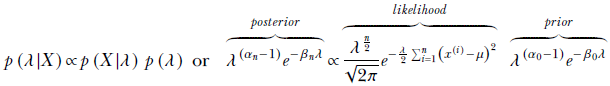
Substituting
and comparing the powers of λ and e, we get
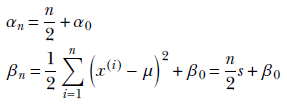
Equation 13.6
Notice that as before, at low values of n, the posterior is dominated by the prior but gets closer and closer to the likelihood estimate as n increases. In other words, in the absence of sufficient data, we let our belief take over the estimation; but if and when data is available, the estimation is dominated by the data-based entity likelihood.
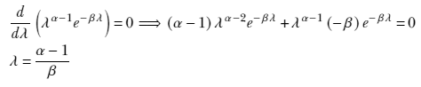
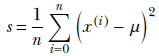
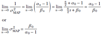
The MAP point estimate for the parameter λ given data set X is obtained by maximizing this posterior distribution p(λ|X) = γ(λ;αn, βn), which yields λMAP = 1/σMAP2 = (αn–1/βn). (Section A.5 in the appendix shows how to obtain the maximum of a gamma distribution.) Thus our estimate for the training data distribution is p(x) = 𝒩(x; μ, σMAP), where 1/σMAP2 = (αn–1/βn).
Given a large volume of data, the MAP estimate for the unknown precision/variance becomes identical to the MLE estimate (proof outline shown):
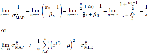
On the other hand, given no data, the MAP estimate for the unknown precision/variance is completely determined by the prior (proof outline shown):
NOTE Fully functional code for Bayesian estimation with a known mean and unknown variance, executable via Jupyter Notebook, can be found at http://mng.bz /2nZ9.
Listing 13.2 PyTorch- Bayesian estimation with unknown variance, known mean
import torch

def inference_unknown_variance(X, prior_dist):
    sigma_mle = torch.std(X)
    n = X.shape[0]

    alpha_0 = prior_dist.concentration
    beta_0 = prior_dist.rate                 ①

    alpha_n = n / 2 + alpha_0
    beta_n = n / 2 * sigma_mle ** 2 + beta_0 ②

    posterior_dist = torch.Gamma(alpha_n, beta_n)
    return posterior_dist
① Parameters of the prior
② Parameters of the posterior
13.7 Fully Bayes parameter estimation: Gaussian, unknown mean, unknown precision
In section 13.3, we saw that if the variance is known, the conjugate prior to the mean is a Gaussian (aka normal) distribution. Likewise, when the mean is known, the conjugate prior to the precision is a gamma distribution. If both are unknown, we end up with a normal-gamma distribution.
13.7.1 Normal-gamma distribution
Normal-gamma is a probability distribution of two random variables, say, μ and λ, whose density is defined in terms of four parameters μ′, λ′, α′, and β′, as follows:

Although it looks complicated, a simple way to remember it is a product of a normal and a gamma distribution.
The normal-gamma distribution attains a maximum at

13.7.2 Estimating the mean and precision parameters
As before, we model the data distribution with a Gaussian: p(x|μ , λ) = 𝒩(x; μ, 1/√λ) we have expressed this Gaussian in terms of the precision, λ, which is related to the variance σ as λ = 1/σ2). The training data set is X = {x(1), x(2),⋯, x(n)}, and its overall likelihood is
We model the prior for the mean as a Gaussian with mean μ0 and precision λ0λ:
![]()
We model the prior for the precision as a gamma distribution with parameters α0, β0:
![]()
The overall prior probability for the mean and precision parameters is the product of the two, a normal-gamma distribution with parameters μ0, λ0, α0, β0:
![]()
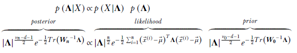
The posterior probability for the mean and precision parameters is the joint (that is, product) of the likelihood and the prior. As such, we know it is another normal-gamma distribution (due to the conjugate prior property of normal-gamma):
![]()
Using Bayes’ theorem,
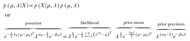
Substituting
and comparing coefficients, the unknown parameters of the posterior distribution can be determined:
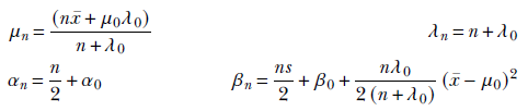
Equation 13.7
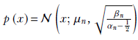
To obtain the fully Bayes parameter estimate, we take the maximum of the normal-gamma posterior probability density function:

Thus the final probability density function for the data is
NOTE Fully functional code for Bayesian estimation with an unknown mean and unknown variance, executable via Jupyter Notebook, can be found at http://mng.bz/1oQy.
Listing 13.3 PyTorch code for a normal-gamma distribution
import torch

class NormalGamma():                            ①


    def __init__(self, mu_, lambda_, alpha_, beta_):
        self.mu_ = mu_
        self.lambda_ = lambda_
        self.alpha_ = alpha_
        self.beta_ = beta_

    @property
    def mean(self):
        return self.mu_, self.alpha_/ self.beta_

    @property
    def mode(self):
        return self.mu_, (self.alpha_-0.5)/ self.beta_
① Since PyTorch doesn’t implement normal-gamma distribution, we implement a bare-bones version.
Listing 13.4 PyTorch: Bayesian estimation with unknown mean, unknown variance
import torch

def inference_unknown_mean_variance(X, prior_dist):
    mu_mle = X.mean()
    sigma_mle = X.std()
    n = X.shape[0]

    mu_0 = prior_dist.mu_
    lambda_0 = prior_dist.lambda_
    alpha_0 = prior_dist.alpha_
    beta_0 = prior_dist.beta_                   ①

    mu_n = (n * mu_mle + mu_0 * lambda_0) / (lambda_0 + n)
    lambda_n = n + lambda_0
    alpha_n = n / 2 + alpha_0
    beta_n = n / 2 * sigma_mle ** 2 + beta_0 +
             0.5* n * lambda_0/ (n + lambda_0) *
             (mu_mle - mu_0) ** 2               ②

    posterior_dist = NormalGamma(mu_n, lambda_n, alpha_n, beta_n)

    return posterior_dist
① Parameters of the prior
② Parameters of the posterior
13.8 Example: Fully Bayesian inferencing
Let’s revisit the problem discussed in section 6.8 of predicting whether a resident of Statsville is female based on height. For this purpose, we have collected height samples from adult female residents of Statsville. Unfortunately, due to unforeseen circumstances, we collected a very small sample. Armed with our knowledge of Bayesian inference, we do not want to let this deter us from trying to build a model. Based on physical considerations, we can assume that the distribution of heights is Gaussian. Our goal is to estimate the parameters (μ, σ) of this Gaussian.
NOTE Fully functional code for this example, executable via Jupyter Notebook, can be found at http://mng.bz/Pn4g.
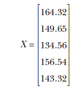
Let’s first create the data set by sampling five points from a Gaussian distribution with μ = 152 and σ = 8. In real-life scenarios, we do not know the mean and standard deviation of the true distribution. But for the sake of this example, let’s assume that the mean height is 152 cm and the standard deviation is 8 cm. Our data matrix, X, is as follows:
13.8.1 Maximum likelihood estimation
If we relied on MLE, our approach would be to compute the mean and standard deviation of the data set and use this normal distribution as our model. We use the following equations to compute the mean and standard deviation of our normal distribution:
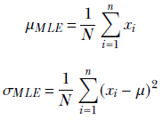
The mean, μ, comes out to be 149.68, and the standard deviation, σ, is 11.52. This differs significantly from the true mean (152) and standard deviation (8) because the number of data points is low. In such low-data scenarios, the maximum likelihood estimates are not very reliable.
13.8.2 Bayesian inference
Can we do better than MLE? One potential method is to use Bayesian inference with a good prior. How do we select a good prior? Well, let’s say that we know from an old survey that the average and standard deviation of the height of adult female residents of Neighborville, the neighboring town, are 150 cm and 9 cm, respectively. Additionally, we have no reason to believe that the distribution of heights at Statsville is significantly different. So we can use this information to “initialize" our prior. The prior distribution encodes our beliefs about the parameter values.
Given that we are dealing with an unknown mean and unknown variance, we model the prior as a normal-gamma distribution:
p(θ) = 𝒩γ(μ0, λ0, α0, β0)
We choose p(θ) such that μ0 = 150, λ0 = 100, α0 = 10.5, and β0 = 810. This implies that
p(θ) = 𝒩γ(150, 100, 10.5, 810)
p(θ|X) is a normal-gamma distribution whose parameters can be computed using equations described in section 13.7. The PyTorch code for computing the posterior is shown next.
Listing 13.5 PyTorch- Computing posterior probability using Bayesian inference
prior_dist = NormalGamma(150, 100, 10.5, 810)                   ①

posterior_dist = inference_unknown_mean_variance(X, prior_dist) ②

map_mu, map_precision =  posterior_dist.mode                    ③

map_std = math.sqrt(1 / map_precision)                          ④

map_dist = Normal(map_mu, map_std)                              ⑤
① Initializes the normal-gamma distribution
② Computes the posterior
③ The mode of the distribution refers to parameter values with the highest probability density.
④ Computes the standard deviation using precision
⑤ map_mu and map_std refer to the parameter values that maximize the posterior distribution.
The MAP estimates for μ and σ obtained using Bayesian inference are 149.98 and 9.56, respectively, which are better than the MLE estimates of 149.68 and 11.52 (the true μ and σ are 152 and 9, respectively).
Now that we’ve estimated the parameters, we can find out the probability that a sample lies in the range using the formula
The details of this can be found in section 6.8.
13.9 Fully Bayes parameter estimation: Multivariate Gaussian, unknown mean, known precision
This is the multivariate case; the univariate version is discussed in section 13.3. The computations follow along the same lines as the univariate ones.
We model the data distribution as a Gaussian p(![]() |
|![]() , Λ) = 𝒩(
, Λ) = 𝒩(![]() ;
; ![]() , Λ−1), where we have expressed the Gaussian in terms of the precision matrix Λ instead of the covariance matrix Σ, where Λ = Σ−1. The training data set is X ≡ {
, Λ−1), where we have expressed the Gaussian in terms of the precision matrix Λ instead of the covariance matrix Σ, where Λ = Σ−1. The training data set is X ≡ {![]() (1),
(1), ![]() (2), ⋯,
(2), ⋯, ![]() (i), ⋯,
(i), ⋯, ![]() (n)}, and its overall likelihood is
(n)}, and its overall likelihood is
![]()
We model the prior for the mean as a Gaussian:
![]()
The posterior probability density is a Gaussian (because it is the product of two Gaussians). Let’s denote it as
![]()
Using Bayes’ theorem,
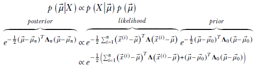
Let’s examine the exponent of the rightmost expression.
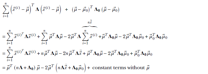
We ignored the last constant terms because they will be rolled into the overall constant of proportionality). Thus
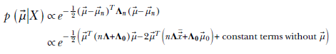
Comparing coefficients:
![]()
The posterior probability maximizes at ![]() n. Thus
n. Thus ![]() MAP =
MAP = ![]() n
n
is the MAP estimate for the mean parameter of the multivariate Gaussian data distribution: p(![]() ) = 𝒩(
) = 𝒩(![]() ;
; ![]() n, Λ-1).
n, Λ-1).
Note the following:
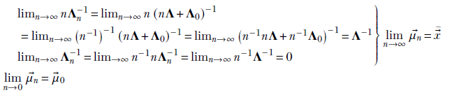
With a large volume of data, the estimated mean parameter ![]() MAP =
MAP = ![]() n approaches the MLE
n approaches the MLE ![]() MLE =
MLE = ![]() .
.
With a low volume of data, the estimated posterior mean parameter ![]() MAP =
MAP = ![]() n approaches the prior
n approaches the prior ![]() 0.
0.
NOTE Fully functional code for multivariate Bayesian inferencing of the mean of a Gaussian likelihood with known precision, executable via Jupyter Notebook, can be found at http://mng.bz/J2AP.
Listing 13.6 PyTorch- Multivariate Bayesian inferencing, unknown mean
def inference_known_precision(X, prior_dist, precision_known):
    mu_mle = X.mean(dim=0)
    n = X.shape[0]


    mu_0 = prior_dist.mean
    precision_0 = prior_dist.precision_matrix       ①


    precision_n = n * precision_known + precision_0 ②
    mu_n = torch.matmul(
        n * torch.matmul(
            mu_mle.unsqueeze(0), precision_known) + torch.matmul(
                mu_0.unsqueeze(0), precision_0),
        torch.inverse(precision_n)
     )

    posterior_dist = MultivariateNormal(
        mu_n, precision_matrix=precision_n)
    return posterior_dist
① Parameters of the prior
② Parameters of the posterior
13.10 Fully Bayes parameter estimation: Multivariate, unknown precision, known mean
In section 13.6, we discussed the univariate case, and now we examine the multivariate case. For the univariate case, we had to look at the gamma distribution. For the multivariate case, we have to look at the Wishart distribution.
13.10.1 Wishart distribution
Suppose we have a Gaussian random data vector ![]() with probability density function 𝒩(
with probability density function 𝒩(![]() ;
; ![]() , Σ). Once again, we use precision matrix Λ instead of the covariance matrix Σ, where Λ = Σ−1. Consider the case where we know the mean
, Σ). Once again, we use precision matrix Λ instead of the covariance matrix Σ, where Λ = Σ−1. Consider the case where we know the mean ![]() but want to estimate the precision Λ. How do we express the prior? Note that p(Λ) is the probability density function of a matrix. So far, we have encountered probability distributions of scalars and vectors, not a matrix. Also, this is not an arbitrary matrix. We are talking about a symmetric, non-negative definite matrix (all covariance and precision matrices belong to this category). Consequently, the distribution we are looking for is not a joint distribution of all the d2 matrix elements d denotes the dimensionality of the data: that is, all
but want to estimate the precision Λ. How do we express the prior? Note that p(Λ) is the probability density function of a matrix. So far, we have encountered probability distributions of scalars and vectors, not a matrix. Also, this is not an arbitrary matrix. We are talking about a symmetric, non-negative definite matrix (all covariance and precision matrices belong to this category). Consequently, the distribution we are looking for is not a joint distribution of all the d2 matrix elements d denotes the dimensionality of the data: that is, all ![]() and
and ![]() vectors are d × 1). Rather, it is a joint distribution of (d(d + 1))/2 elements in the matrix—the diagonal and those above or below (diagonal elements above and below are identical because the matrix is symmetric).
vectors are d × 1). Rather, it is a joint distribution of (d(d + 1))/2 elements in the matrix—the diagonal and those above or below (diagonal elements above and below are identical because the matrix is symmetric).
The space of such matrices is called a Wishart ensemble. The probability of a random-precision matrix Λ of size d × d can be expressed as a Wishart distribution. This distribution has two parameters:
-
ν, a scalar, satisfying ν > d − 1
-
W, a d × d symmetric non-negative definite matrix
The probability density function is
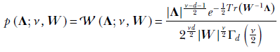
where
-
𝒲 denotes Wishart.
-
|W|, |Λ| denote the determinants of the matrices W and Λ, respectively.
-
Tr(A) denotes the trace of a matrix A (sum of the diagonal elements).
-
Γ denotes the multivariate gamma function
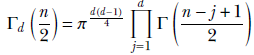
The Wishart is the multivariate version of the gamma distribution. Its expected value is
𝔼(Λ) = νW
Its maxima occur at
Λ = (ν − d − 1)W for ν ≥ d + 1
13.10.2 Estimating precision
As before, we model the data distribution as a Gaussian p(![]() |
|![]() , Λ) = 𝒩(
, Λ) = 𝒩(![]() ;
; ![]() , Λ−1), where we have expressed the Gaussian in terms of the precision matrix Λ instead of the covariance matrix Σ, where Λ = Σ−1.
, Λ−1), where we have expressed the Gaussian in terms of the precision matrix Λ instead of the covariance matrix Σ, where Λ = Σ−1.
The training data set is X ≡ {![]() (1),
(1), ![]() (2),⋯,
(2),⋯, ![]() (i),⋯,
(i),⋯, ![]() (n)}, and its overall likelihood is
(n)}, and its overall likelihood is
![]()
We model the prior probability of the precision matrix as a Wishart distribution. Hence,
![]()
The posterior is another Wishart (owing to the Wishart conjugate prior property):
![]()
Using Bayes’ theorem for the training data set X,
Let’s study a pair of simple lemmas that will come in handy.
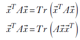
where Tr refers to Trace of a matrix (sum of diagonal elements).
-
The first lemma is almost trivial—the quadratic form
 TA is a scalar, so of course it is the same as its trace.
 -
The second lemma follows directly from the matrix property of a trace: Tr(BC) = Tr(CB).
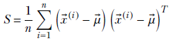
Using the lemmas, the exponent of the likelihood term is
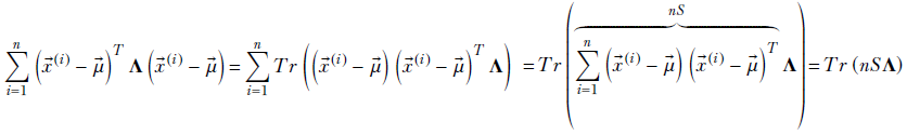
where
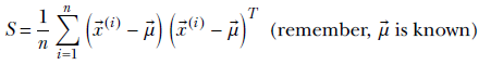
Thus, the posterior density is
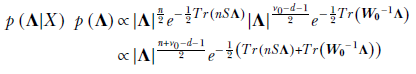
Since Tr(A) + Tr(B) = Tr(A + B),
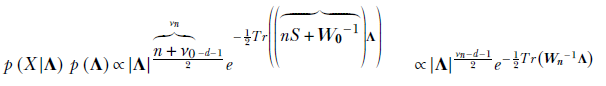
Comparing coefficients, we determine the unknown parameters of the posterior distribution:
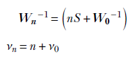
where
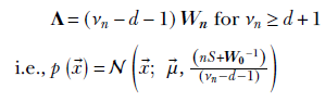
The maximum of the posterior density function, 𝒲(Λ;νn, Wn), ields an estimate for the precision parameter of the data distribution: Λ = (νn − d − 1)Wn for νn ≥ d + 1 i.e.,
Summary
-
A generative model that models the underlying data distribution can be more powerful than a black box discriminative model. Once we choose a model family, we need to estimate the model parameters, θ. We can estimate the best values of θ from the training data X using Bayes’ theorem.
-
The posterior distribution p(θ|X) is a function of the product of likelihood p(X|θ) and the prior p(θ). The prior expresses our belief in the value of the parameters. The posterior is dominated by the prior for small data sets and the likelihood for large data sets. Injecting belief via a good prior distribution can be helpful in settings with very little training data.
-
Maximum likelihood estimation only relies on the data, in contrast to maximum a posteriori (MAP) estimation, which relies on the data as well as the prior information.
-
We can use Bayesian estimation for the mean of a Gaussian likelihood when the variance is known. When the likelihood is Gaussian p(X) ∼ N(μ, σ), we model the prior as a normal distribution p(μ) ∼ N(μ0, σ0). The posterior distribution is also a normal distribution p(μ|X) ∼ N(μn, σn), where
 and
and 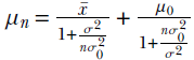 . We can also use the estimated parameter to make predictions about new instances of data.
 -
Weak priors imply a high degree of uncertainty/lower confidence in our prior belief and can easily be overwhelmed by the data. In contrast, strong priors imply a lower degree of uncertainty/higher confidence in our prior belief and will resist data overload.
-
For a specific family of likelihood, the choice of the prior that results in the posterior belonging to the same family as the prior is called a conjugate prior.
-
The gamma function is
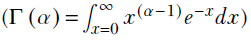 , and the gamma distribution is
 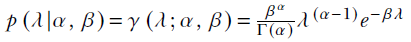 . The gamma distribution varies with different values of α and β.
 -
In the case of Bayesian estimation of the precision of the Gaussian likelihood for a known mean, the precision λ is the inverse of the variance. We can model the prior as a gamma distribution
 . The posterior distribution is also a gamma distribution,
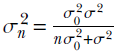
 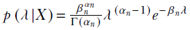 , where
 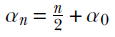 and
and 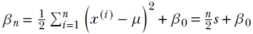 .
. -
In Bayesian estimation of both the mean and precision of a Gaussian likelihood, we model the prior as a normal-gamma distribution. The posterior is another normal-gamma distribution. The posterior distribution can be used to predict new data instances.
-
The multivariate setting of Bayesian inferencing of the mean of a Gaussian likelihood is known as precision. We can model the prior as a multivariate normal distribution; the posterior is also a multivariate normal distribution.
-
The Wishart distribution is the multivariate version of the gamma distribution. With multivariate Bayesian inferencing of the precision of a Gaussian likelihood with a known mean, we can model the prior as a Wishart distribution. The corresponding posterior is also a Wishart distribution.