14 Latent space and generative modeling, autoencoders, and variational autoencoders
This chapter covers
- Representing inputs with latent vectors
- Geometrical view, smoothness, continuity, and regularization for latent spaces
- PCA and linear latent spaces
- Autoencoders and reconstruction loss
- Variational autoencoders (VAEs) and regularizing latent spaces
Mapping input vectors to a transformed space is often beneficial in machine learning. The transformed vector is called a latent vector—latent because it is not directly observable—while the input is the underlying observed vector. The latent vector (aka embedding) is a simpler representation of the input vector where only features that help accomplish the ultimate goal (such as estimating the probability of an input
belonging to a specific class) are retained, and other features are forgotten. Typically, the latent representation has fewer dimensions than the input: that is, encoding an input into a latent vector results in dimensionality reduction.
The mapping from input to latent space (and vice versa) is usually learned—we train a machine, such as a neural network, to do it. The latent vector needs to be as faithful a representation as possible of the input within the dimensionality allocated to it. So, the neural network is incentivized to minimize the loss of information caused by the transformation. Later, we see that in autoencoders, this is achieved by reconstructing the input from the latent vector and trying to minimize the difference between the actual and reconstructed input. However, given the reduced number of dimensions, the network does not have the luxury of retaining everything in the input. It has to learn what is essential to the end goal and retain only that. Thus the embedding is a compact representation of the input that is streamlined to achieve the ultimate goal.
14.1 Geometric view of latent spaces
Consider the space of all digital images of height H, width W, with each pixel representing a 24-bit RGB color value. This is a gigantic space with (224)HW points. Every possible RGB × H × W image is a point in this space. But if an image is a natural image, neighboring points tend to have similar colors. This means points corresponding to natural images are correlated: they are not distributed uniformly over the space of possible images. Furthermore, if the images have a common property (say, they all giraffes), the corresponding points form clusters in the (224)HW-sized input space. In stochastic parlance, the probability distribution of natural images with a common property over the space of possible images is highly non-uniform (low entropy).
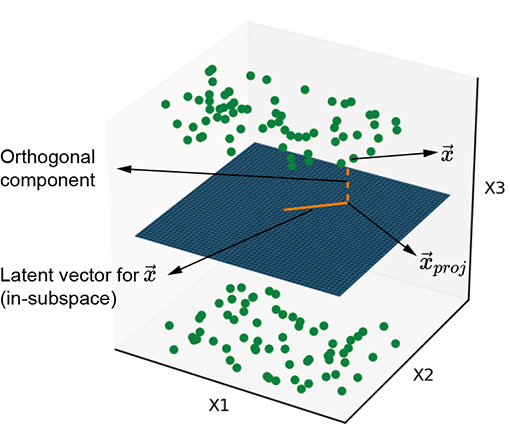
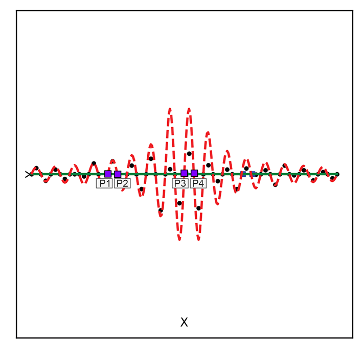
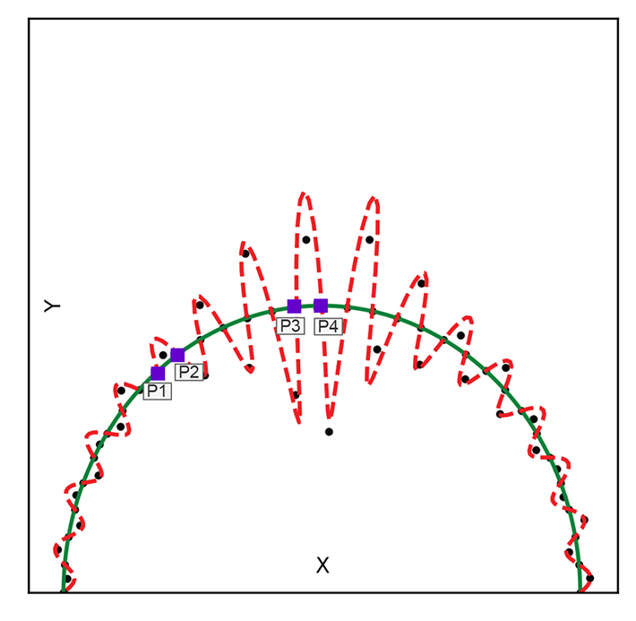
Figure 14.1a illustrates points with some common property clustered around a planar manifold. Similarly, figure 14.1b illustrates points with some common property clustered around a curved manifold. These points have a common property. At the moment, we are not interested in what that property is or whether the manifold is planar or curved. All we care about is that these points of interest are distributed around a manifold. The manifold captures the essence of that common property, whatever it is. If the common property is, say, the presence of a giraffe in the image, then the manifold captures giraffeness: the points on or near the manifold all correspond to images with giraffes. If we travel along the manifold, we encounter various flavors of giraffe photos. If we go far from the manifold—that is, travel a long distance in a direction orthogonal to the manifold—the probability of the point representing a photo with a giraffe is low.
(a) Planar latent subspaces
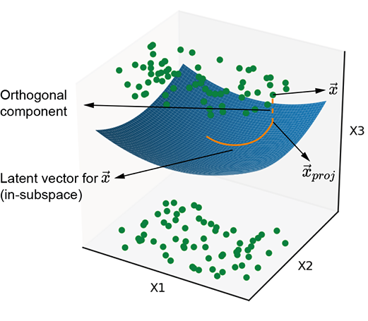
(b) Curved latent subspace
Figure 14.1 Two examples of latent subspaces, with planar and curved manifolds, respectively. The solid line shows the latent vector, and the dashed line represents the information lost by projecting onto the latent subspace.
Given training data consisting of sampled points of interest (such as many giraffe photos), we can train a neural network to learn this manifold—it is the optimal manifold that minimizes the average distance of all the training data points from the manifold. Then, at inference time, given an arbitrary input point, we can estimate its distance from the manifold, giving us the probability of that input satisfying the property represented by the manifold.
Thus, the input vector can be decomposed into an in-manifold component (solid line in figure 14.1) and an orthogonal-to-manifold component (dashed line in figure 14.1). Latent space modeling effectively eliminates the orthogonal component and retains the in-manifold component as the latent vector (aka embedding). Equivalently, we are projecting the input vector onto the manifold. This is the core idea of latent space modeling—we learn a manifold that represents a property of interest and represents all inputs by a latent vector, which is the input point’s projection onto this manifold. The latent vector is a more compact representation of the input where only information related to the property of interest is retained.
A subtle point is that the latent vector is the in-manifold component of the original point’s position vector. By switching to the latent vector representation, we lose the location of the point in the original higher-dimensional input space. We can go back to the higher-dimensional space by providing the location of the manifold for the lost orthogonal component, but doing so does not recover the original point: it recovers only the projection of the original point onto the subspace. We are replacing the individual orthogonal components with an aggregate entity the location of a manifold) but do not recover the exact original point. Some information is irretrievably lost during projection.
A special case of latent space representation is principal component analysis (PCA), introduced in section 4.4 (section 14.4 provides a contextual recap of PCAs). It projects input points to an optimal planar latent subspace (as in figure 14.1a). But except for some lucky special cases, the best latent subspace is not a hyperplane. It is a complex curved surface (see figure 14.1b). Neural networks, such as autoencoders, can learn such nonlinear projections.
14.2 Generative classifiers
During inferencing, the supervised classifiers we have encountered in previous chapters typically emit the class to which an input belongs, perhaps along with a bounding box. This is somewhat black-box-like behavior. We do not know how well the classifier has mastered the space except through the quantized end results. Such classifiers are called discriminative classifiers. On the other hand, latent space models map arbitrary input points to probabilities of belonging to the class of interest. Such models are called generative models, and they have some desirable properties:
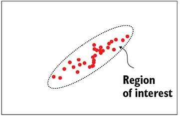
(a) A good discriminative classifier—smooth decision boundary
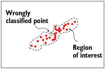
(b) A bad discriminative classifier—irregular decision boundary
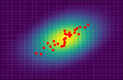
(c) Generative model—no decision boundary (heat map indicates the probability density)
Figure 14.2 Solid circles indicate training data points (all belonging to the class of interest). The dashed curve indicates the decision boundary separating the class of interest from the class of non-interest. In a generative model, there is no decision boundary. Every point in the space is associated with a probability of belonging to the class of interest (indicated as a heat map in figure 14.2c)
NOTE We can always create a discriminative classifier from a generative classifier by putting a threshold on the probability.
-
Smoother, denser manifolds—Discriminative models learn decision boundaries separating data points of interest from those not of interest in the input space. On the other hand, generative models try to model the distribution of the data points of interest in the input space using smooth probability density functions. As such, the generative model can't learn a very irregularly shaped function that overfits the training data. This is illustrated in figure 14.2, whereas the discriminative model may converge to a manifold that follows the nooks and bends of the training data too closely (overfits) as in figure~\ref{fig-discriminative-bad-model}. This difference between discriminative and generative classifiers becomes especially significant when we have less training data. We can always create a discriminative classifier from a generative classifier by putting a threshold on the probability.
-
Extra insight—Generative models offer more insight into the inner workings of the model. Consider a model that recognizes horses. Suppose we feed some horse images to the model, and it calls them horses (good). Then we feed the model some zebra images, and it calls them horses, too (bad). Do we have a useless~model that calls everything a horse? If it is a discriminative model, we must test it with totally different images (say, bird images) to get the answer. But if we have a generative model, it says the probabilities of the true horse images are, say, 0.9 and above, while the probabilities for the zebra images are around 0.7. We begin to see that the model is behaving reasonably and does realize that zebras are less "horsy" than real horses.
-
New class instances—A generative model learns the distribution of input points belonging to the class. An advantage related to learning the distribution is that we can sample the distribution to generate new members of the class (for example, to generate artificial horse images). This leads to the name generative modes. If we train a generative model with writings of Shakespeare, it will emit Shakespeare-like text pieces. Believe it or not, this has been tried with some success.
14.3 Benefits and applications of latent-space modeling
Let’s recap at a high level why we want to do latent-space modeling:
-
Generative models are often based on latent space models—all the benefits of generative modeling as outlined in section 14.2 apply to latent space modeling too.
-
Attention to what matters—Redundant information that does not contribute to the end goal is eliminated, and the system focuses on truly discriminative information. To visualize this, imagine an input data set of police mugshots consisting of people standing in front of the same background. Latent-space modeling trained to recognize people typically eliminates the common background from the representation and focuses on the photograph’s subject matter (people).
-
Streamlined representation of data—The latent vector is a more compact representation of the input vector (reduced dimensions and hence smaller) with no meaningful information lost.
-
Noise elimination—Latent-space modeling eliminates the low-variance orthogonal-to-latent-subspace component of the data. This is mostly data that does not help in the problem of interest and hence is noise.
-
Transformation to a manifold that is friendlier toward the end goal—We have seen this notion previously, but here let’s look at an interesting simple example. Consider a set of 2D points in Cartesian coordinates (x, y). Suppose we want to classify the points into two sets: those that lie inside the circle x2 + y2 = a2 and those that lie outside the circle. In the original Cartesian space, the decision boundary is not linear (it is circular). But if we transform the Cartesian input points to a latent space in polar coordinates—that is, each (x, y) is mapped to (r, θ) such that x = rcos(θ), y = rsin(θ)—the circle transforms into a line r = a in the latent space . A simple linear classifier r = a in the latent space can achieve the desired classification.
Some applications of latent-space modeling are as follows:
-
Generating artificial images or text (as explained in the context of generative modeling).
-
Similarity estimation between inputs—If we map inputs to latent vectors, we can assess the similarity between inputs by computing the Euclidean distance between the latent vectors. Why is this better than taking the Euclidean distance between the input vectors? Suppose we are building a recommendation engine that suggests other clothing items “similar” to the one a potential buyer is currently browsing. We want to retrieve other clothing items that look similar but not identical to the one viewed. But similarity is a subjective concept, not quite measurable via the similarity of the inputs’ pixel colors. Consider a shirt with black vertical stripes on a white base. If we switch the stripe color with the base color, we get a shirt with white vertical stripes on a black base. If we do pixel-to-pixel color matching, these are very different, yet they are considered similar by humans. For this problem, we have to train the latent space model, creating neural networks so that images perceived to be similar by humans map to points in latent space that are close to each other. For example, both white-on-black and black-on-white shirts should map to latent vectors that are close to each other in the latent space even though they are far apart in the input space.
-
Image or other data compression—The latent vector approximates the data with a smaller-dimensional vector that mimics the original vector as faithfully as possible. Thus the latent vector is a lossy compressed representation of the input.
-
Denoising—The latent vector eliminates the non-meaningful part of the input information, which is noise.
NOTE Fully functional code for this chapter, executable via Jupyter Notebook, can be found at http://mng.bz/6XG6.
14.4 Linear latent space manifolds and PCA
PCAs (which we discussed in section 4.4) project input data onto linear hyperplanar manifolds. Revisiting this topic will set up the correct context for the rest of this chapter. Consider a set of 3D input data points clustered closely around the X0 = X2 plane, as shown in figure 14.3.
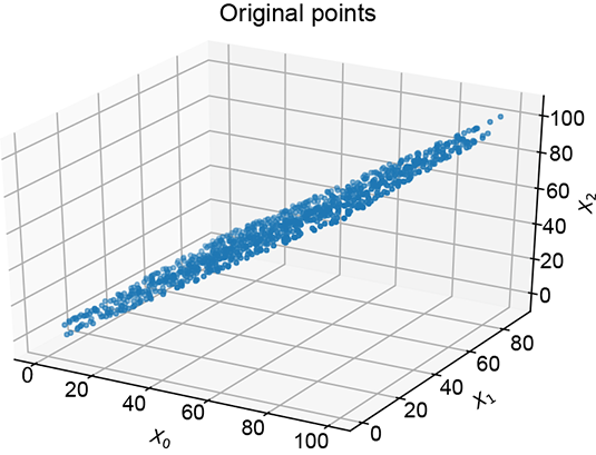
(a) Original 3D data
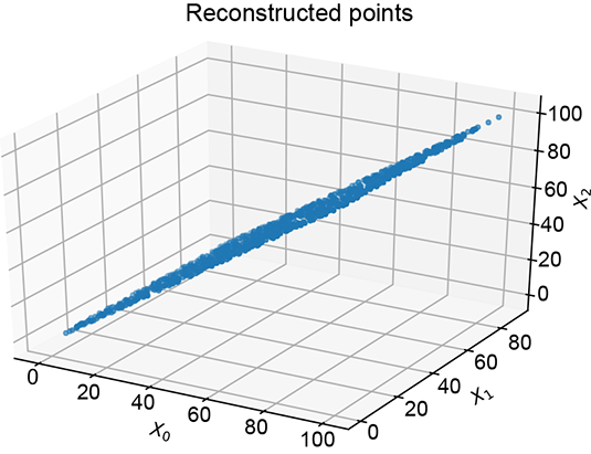
(b) Lower-dimensional 2D representation obtained by setting the third principal value to zero
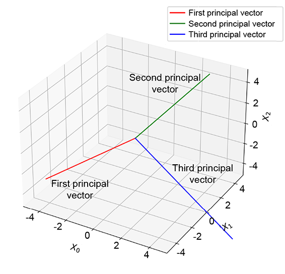
(c) The principal vectors of the original data. The third principal vector is normal to X0 = X2 plane; the other two are in-plane.
Figure 14.3 The original 3D data in figure 14.3a shows high correlation: points are clustered around the X0 = X2 plane. The first principal component corresponds to the direction of maximum variance. The last (third) principal reduced to a 2D latent vector.
NOTE We denote the successive axes (dimensions) as X0, X1, X2 instead of the more traditional X, Y, Z for easy extension to higher dimensions.
Using PCA, we can recognize that the data has low variation along some dimensions. When we do PCA, we get the principal value and principal vector pairs. The largest principal value corresponds to the direction of maximum variance in the data. The corresponding principal vector yields that direction, and that principal value indicates the magnitude of the variance along that direction. The next principal value, the principal vector pair, is the orthogonal direction with the next-highest variance, and so on. For instance, in figure 14.3, the principal vectors corresponding to the larger two principal values lie in the X0 = X2 plane, while the smallest principal value corresponds to the normal-to-plane vector. The third principal value is significantly smaller than the others. This tells us that variance along that axis is low, and components along that axis can be dropped with relatively little loss of information: that is, low reconstruction loss. The variations along the small principal value axes are likely noise, so eliminating them cleans up the data. In figure 14.3, this effectively projects the data onto the X0 = X2 plane.
Following are the steps involved in PCA-based dimensionality reduction. This was described in detail with proofs in section 4.5; here we recap the main steps without proof.
NOTE This treatment is similar but not identical to that in section 4.5. Here we have switched the variables m and n to be consistent with our use of n to denote the data instance count. We have also switched to a slightly different flavor of the SVD.
-
Represent the data as a matrix X, where each row is an individual data instance. The number of rows n is the size of the data set. The number of columns d is the original (input) dimensionality of the data. Thus X is a n × d matrix.
-
Compute the mean data vector
where (i) for i = 1 to i = n denote the training data vector instances (which form rows of the matrix X).
 -
Shift the origin of the coordinate system to the mean by subtracting the mean vector from each data vector:
(i) = (i) –  for all i
The data matrix X now has the mean-subtracted data instances as rows. -
The matrix XTX where X is the mean-subtracted data matrix) is the covariance matrix (as discussed in detail in section 5.7.2). The eigenvalue, eigenvector pairs of the matrix XTX are known as principal values and principal vectors (together referred to as principal components). Since XTX is a d × d matrix, there are d scalar eigenvalues and d eigenvectors, each of dimension d × 1. Let’s denote the principal components as (λ1,
 1), (λ2, 2), ⋯, (λdm, d).
 -
We can assume λ1 ≥ λ2 ≥ ⋯ ≥ λd if necessary, we can make this true by renumbering the principal components). Then the first principal component corresponds to the direction of maximum variance in the data (proof with geometrical intuition can be found in section 5.7.2). The corresponding principal value yields the actual variance. The next principal value corresponds to the second-highest variance (among directions orthogonal to the first principal direction), and so forth. For every component, the principal value yields the actual variance, and the principal vector yields the direction.
-
Consider the matrix of principal vectors:
V = [1 2 … d]
If we want the data to be a space with m dimensions with minimal loss of information, we should drop the last m vectors of V. This eliminates the m least-variance dimensions. Dropping the last m vectors from V yields a matrix
Vd–m = [1 2 … d–m]
Note that the best way to obtain the V matrix is to perform SVD on the mean-subtracted X (see section 4.5). -
Premultiplying Vd−m, the truncated principal vectors matrix, with the original data matrix X projects the data onto a space corresponding to the first d − m principal components. Thus, to create d − m-dimensional linearly encoded latent vectors from d-dimensional data,
Xd−m = XVd−m
Xd−m is the reduced dimension data set. Its dimensionality is n × (d−m).
It can be shown that
XVd−m = UΣd−m
where U is from SVD (see section 4.5) and Σd−m is a truncated version of the diagonal matrix Σ from SVD with its smallest m elements chopped off. This offers an alternative way to do PCA-based dimensionality reduction. -
How do we reconstruct? In other words, what is the decoder? Well, to reconstruct, we need to save the original principal vectors: that is, the V matrix. If we have that, we can introduce m zeros at the right of every row in Xd−m to make it a n × d matrix again. Then we post-multiply by VT, which rotates the coordinate system back from one with principal vectors as axes to one with the original input axes. Finally, we add the mean
to each row to shift the origin back to its original position, which yields the reconstructed data matrix X̃. The reconstruction loss is ||X − X̃||2. Note that, in effect, X̃ is UΣVT with the last m diagonal elements of Σ set to zero. -
The reconstructed data X̃ is not identical to the original data. The information we lost during dimensionality reduction the normal-to-plane components) is lost permanently. Nonetheless, this principled way of dropping information ensures that the reconstruction loss is minimal in some sense, at least among all X̃ linearly related to X.
14.4.1 PyTorch code for dimensionality reduction using PCA
Now, let’s implement dimensionality reduction in PyTorch. Let X be a data matrix representing points clustered around the X0 = X2 plane. X is of shape [1000,3], with each row of X representing a three-dimensional data point. The following listing shows how to project X into a lower-dimensional space with minimal loss of information. It also shows how to reconstruct the original data points from the lower-dimensional representations. Note that the reconstructions are approximate because we have lost information (albeit minimal) in the dimensionality-reduction process.
NOTE Fully functional code for dimensionality reduction using PCA, executable via Jupyter Notebook, can be found at http://mng.bz/7yJg.
Listing 14.1 PyTorch- PCA revisited
import torch

X = get_data()                                      ①

X_mean = X.mean(axis=0)                             ②

X = X - X_mean                                      ③

U, S, Vh = torch.linalg.svd(X, full_matrices=False) ④

V = Vh.T                                            ⑤

V_trimmed =  V[:, 0: 2]                             ⑥

X_proj = torch.matmul(X, V_trimmed)                 ⑦

X_proj = torch.cat([X_proj,                         ⑧
              torch.zeros((X_proj.shape[0], 1))], axis=1)

X_recon = torch.matmul(X_proj, Vh)                  ⑨

X_recon = X_recon + X_mean                          ⑩
① Data matrix of shape (1000, 3)
② Stores the mean so we can reconstruct the original data points later
③ Subtracts the mean before performing SVD
④ Runs SVD
⑤ Columns of V are the principal vectors.
⑥ Removes the last principal vector. This is along the direction of least variance perpendicular to X0 = X2 plane).
⑦ Projects the input data points into the lower-dimensional space
⑧ Pads with zeros to make an n × d matrix
⑨ Post-multiplies with VT to project back to the original space
⑩ Adds the mean
14.5 Autoencoders
Autoencoders are neural network systems trained to generate latent-space representations corresponding to specified inputs. They can do nonlinear projections and hence are more powerful than PCA systems see figure 14.4). The neural network mapping the input vector to a latent vector is called an encoder. We also train a neural network called a decoder that maps the latent vector back to the input space. The decoder output is the reconstructed input from the latent vector. The reconstructed input (that is, the output of the decoder) will never match the original input exactly—information was lost during encoding and cannot be brought back—but we can try to ensure that they match as closely as possible within the constraints of the system. The reconstruction loss is a measure of the difference between the original input and the reconstructed input. The encoder-decoder pair is trained end to end to minimize reconstruction loss (along with, potentially, some other losses). This is an example of representation learning, whereby we learn to represent input vectors with smaller latent vectors representing the input as closely as possible in the stipulated size budget. The budgeted size of the latent space is a hyperparameter.
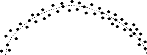
Figure 14.4 A 2 data distribution with a curved underlying pattern. It is impossible to find a straight line or vector such that all points are near it. PCA will not do well.
NOTE A hyperparameter is a neural network parameter that is not learned. Its value is set based on our knowledge of the system and held constant during training.
The desired output is implicitly known in autoencoders: it is the input. Consequently, no human labeling is needed to train autoencoders; they are unsupervised. An autoencoder is shown schematically in figure 14.5.
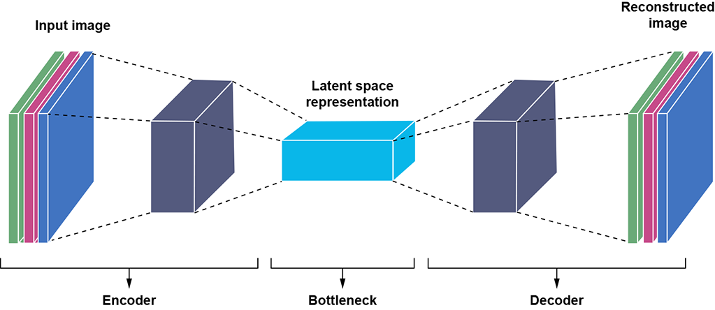
Figure 14.5 Schematic representation of an autoencoder. The encoder transforms input into a latent vector. The decoder transforms the latent vector into reconstructed input. We minimize the reconstruction loss—the distance between the reconstructed input and the original input.
-
The encoder takes an input
and maps it to a lower-dimensional latent vector  . An example of an encoding neural network for image inputs is shown in listing 14.2. Note how the image height and width keep decreasing with each successive sequence of convolution, ReLU, and max pool layers.
 -
The decoder is a neural network that generates reconstructed image
 from the latent vector . Listing 14.3 shows an example of a decoder neural network. Note the transposed convolutions and how the height and width of the image keep increasing with each successive sequence of transposed convolution, batch normalization, and ReLU. Transposed convolutions are discussed in section 10.5.) The decoder essentially remembers—not exactly, but in an average sense—the information discarded during encoding. Equivalently, it remembers the position of the latent space manifold in the overall input space. Adding that back to the latent space representation takes us back to the same dimensionality as the input vector but not to the same input point.
 -
The system minimizes the information loss from the encoding (the reconstruction loss). We are ensuring that for each input, the corresponding latent vector produced by the encoder can be mapped back to a reconstructed value by the decoder that is as close as possible to the input. Equivalently, each latent vector is a faithful representation of the input, and there is a 1 : 1 mapping between inputs and latent vectors.
-
The encoder and decoder need not be symmetric.
Mathematically,
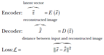
The end-to-end system is trained to minimize the loss ℒ.
NOTE Fully functional code for autoencoders, executable via Jupyter Notebook, can be found at http://mng.bz/mOzM.
Listing 14.2 PyTorch- Autoencoder encoder
from torch import nn
nz = 10
input_image_size = (1, 32, 32)            ①
conv_encoder = nn.Sequential(
            nn.Conv2d(in_channels, 32, kernel_size=3, stride=1, padding=1),
            nn.BatchNorm2d(32),
            nn.ReLU(),
            nn.MaxPool2d(kernel_size=2),  ②
            nn.Conv2d(32, 128, kernel_size=3, stride=1, padding=1),
            nn.BatchNorm2d(128),
            nn.ReLU(),
            nn.MaxPool2d(kernel_size=2),  ③
            nn.Conv2d(128, 256, kernel_size=3, stride=1, padding=1),
            nn.BatchNorm2d(256),
            nn.ReLU(),
            nn.MaxPool2d(kernel_size=2),  ④

            nn.Flatten()                  ⑤
        )
fc = nn.Linear(4096, nz)                  ⑥
① Input image size in (c, h, w) format
② Reduces to a (32, 16, 16)-sized tensor
③ Reduces to a (128, 8, 8)-sized tensor
④ Reduces to a (256, 4, 4)-sized tensor
⑤ Flattens to a 4096-sized tensor
⑥ Reduces the 4096-sized tensor to an nz-sized tensor
Listing 14.3 PyTorch- Autoencoder decoder
from torch import nn
decoder = nn.Sequential(
            nn.ConvTranspose2d(self.nz, out_channels=256,
             kernel_size=4, stride=1,
             padding=0, bias=False),            ①

            nn.BatchNorm2d(256),
            nn.ReLU(True),
            nn.ConvTranspose2d(256, 128, kernel_size=2,
              stride=2, padding=0, bias=False), ②
            nn.BatchNorm2d(128),
            nn.ReLU(True),
            nn.ConvTranspose2d(128, 32, kernel_size=2,
              stride=2, padding=0, bias=False), ③
            nn.BatchNorm2d(32),
            nn.ReLU(True),
            nn.ConvTranspose2d(32, in_channels, kernel_size=2,
              stride=2, padding=0, bias=False), ④
            nn.Sigmoid()
        )
① Converts (nz, 1, 1) to a 256, 4, 4)-sized tensor
② Increases to a 128, 8, 8)-sized tensor
③ Increases to a 32, 16, 16)-sized tensor
④ Increases to a 1, 32, 32)-sized tensor
Listing 14.4 PyTorch- Autoencoder training
from torch import nn
from torch.nn import functional as F

conv_out = conv_encoder(X)     ①

z =  fc(conv_out)              ②
Xr = decoder(z)                ③

recon_loss = F.mse_loss(Xr, X) ④
① Passes the input image through the convolutional encoder
② Reduces to nz dimensions
③ Reconstructs the image using z via the decoder
④ Computes the reconstruction loss
14.5.1 Autoencoders and PCA
It is important to realize that autoencoders perform a much more powerful dimensionality reduction than PCA. PCA is a linear process; it can only project data points to best-fit hyperplanes. Autoencoders can fit arbitrary complex nonlinear hypersurfaces to the data, limited only by the expressive powers of the encoder-decoder pair. If the encoder and decoder have only a single linear layer (no ReLU or other nonlinearity), then the autoencoder projects the data points to a hyperplane like PCA not necessarily the same hyperplane).
14.6 Smoothness, continuity, and regularization of latent spaces
Minimizing the reconstruction loss does not yield a unique solution. For instance, figure 14.6 shows two examples of transforming 2D inputs into 1D latent-space representations, linear and curved, respectively. Both the regularized solid line) and the non-regularized zigzag manifold (dashed line) fit the training data well with low reconstruction error. But the former is smoother and more desirable.
(a) Linear latent space
(b) Curved latent space
Figure 14.6 Two examples of mapping from a 2D input space to a 1D latent space. Both show regularized solid) vs. unregularized (dashed) latent space manifolds. Solid little circles depict training data points.
Note the pair of points marked p1, p2 and p3, p4(square markers). The distance between them is more or less the same in the input space. But when projected on the dashed curve (unregularized latent space), their distances (measured along the curve) become quite different. This is undesirable and does not happen in the regularized latent space (here, the distance is measured along a solid line). It becomes much more pronounced in high dimensions.
The zigzag curve segment containing the training data set is longer than the smooth one. A good latent manifold typically has fewer twists and turns (is smooth) and hence has a “length” that is minimal in a sense. This is reminiscent of the minimum descriptor length (MDL) principle, which we discussed in section 9.3.1.
How do we ensure that this smoothest latent space is chosen over others that also minimize the reconstruction loss? By putting additional constraints (losses) over and above the ubiquitous reconstruction loss. Recall the notion of regularization, which we looked at in sections 6.6.3 and 9.3. There we introduced an explicit loss that penalizes longer solutions (which was equivalent to maximizing the a posteriori probability of parameter values as opposed to the likelihood). A related approach that we explore in this chapter is to model the latent space as a probability distribution belonging to a known family (for example, Gaussian) and minimize the difference (KL divergence) of this estimated distribution from a zero-mean univariance Gaussian. The encoder-decoder neural network pair is trained end to end to minimize a loss that is a weighted sum of the reconstruction loss and this KL divergence. Trying to remain close to the zero-mean unit-variance Gaussian penalizes departure from compactness and smoothness. This is the basic idea of variational autoencoders VAEs).
The overall effect of regularization is to create a latent space that is more compact. If we only minimize the reconstruction loss, the system can achieve that by mapping points very far from each other (space being infinite). Regularization combats that and incentivizes the system to not map the training points too far from one another. It tries to limit the total latent-space volume occupied by the points corresponding to the training inputs.
14.7 Variational autoencoders
VAEs are a special case of autoencoders. They have the same architecture: a pair of neural networks that encode and decode the input vector, respectively. They also have the reconstruction loss term. But they have an additional loss term called KL divergence loss that we explain shortly.
NOTE Throughout this chapter, we denote latent variables with ![]() and input variables with
and input variables with ![]() .
.
14.7.1 Geometric overview of VAEs
Figure 14.7 attempts to provide a geometrical view of VAE latent-space modeling. During training, given an input ![]() , the encoder does not directly emit the corresponding latent-space representation
, the encoder does not directly emit the corresponding latent-space representation ![]() . Instead, the encoder emits the parameters of a distribution from a prechosen family. For instance, if the prechosen family is Gaussian, the encoder emits a pair of parameter values
. Instead, the encoder emits the parameters of a distribution from a prechosen family. For instance, if the prechosen family is Gaussian, the encoder emits a pair of parameter values ![]() (
(![]() ), Σ(
), Σ(![]() ). These are the mean and covariance matrix of a specific Gaussian distribution 𝒩(
). These are the mean and covariance matrix of a specific Gaussian distribution 𝒩(![]() ;
; ![]() (
(![]() ), Σ(
), Σ(![]() )) in the latent space. The latent-space representation
)) in the latent space. The latent-space representation ![]() corresponding to the input
corresponding to the input ![]() is obtained by sampling this distribution emitted by the encoder. Thus in the Gaussian case, we have
is obtained by sampling this distribution emitted by the encoder. Thus in the Gaussian case, we have ![]() ∼ 𝒩(
∼ 𝒩(![]() ;
; ![]() (
(![]() ), Σ(
), Σ(![]() )).
)).
NOTE The symbol ∼ indicates sampling from a distribution.
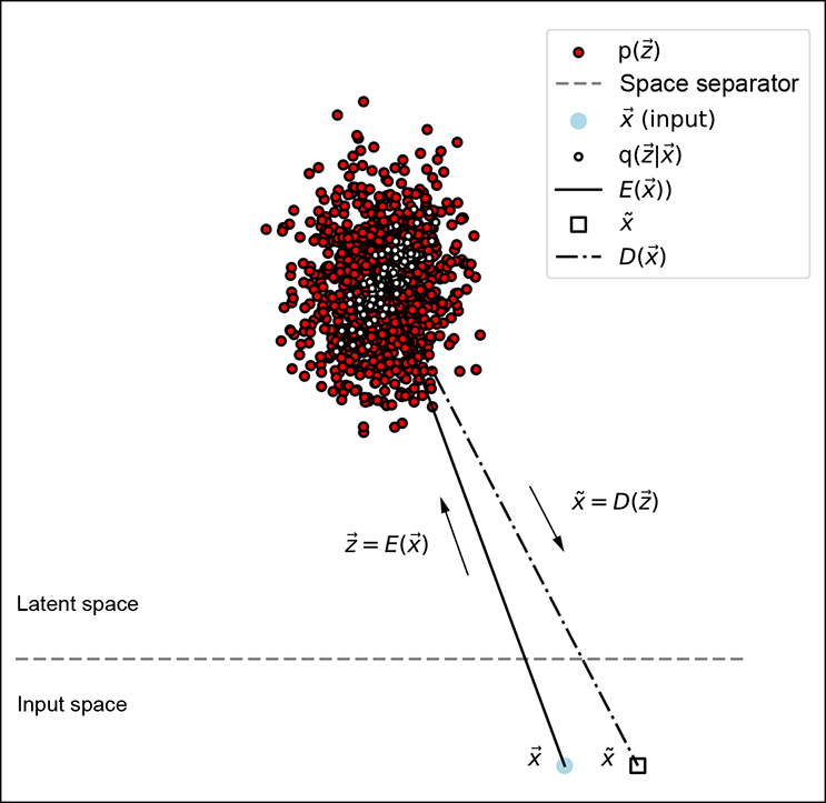
Figure 14.7 Geometric depiction of VAE latent-space modeling distributions
This distribution, which we call the latent-space map of the input ![]() , is shown by hollow circles with dark borders in figure 14.7. Such mapping is called stochastic mapping.
, is shown by hollow circles with dark borders in figure 14.7. Such mapping is called stochastic mapping.
The latent-space map distribution should have a narrow, single-peaked probability density function (for example, a Gaussian with small variance: that is, small ||Σ||). The narrow-peakedness of the probability density function implies that the cloud of sample points forms a tight, small cluster—any random sample from the distribution will likely be close to the mean. So, sampling ![]() from such a distribution is not very different from a deterministic mapping from
from such a distribution is not very different from a deterministic mapping from ![]() to
to ![]() =
= ![]() (
(![]() ). This sampling to obtain the latent vector is done only during training. During inferencing, we use the mean emitted by the encoder directly as the latent-space representation of the input: that is,
). This sampling to obtain the latent vector is done only during training. During inferencing, we use the mean emitted by the encoder directly as the latent-space representation of the input: that is, ![]() =
= ![]() (
(![]() ).
).
The decoder maps the latent vector representation ![]() back to a point, say x̃, in the input space. This is the reconstructed version of the input vector (shown by a little white square with a black border in figure 14.7). The decoder is thus estimating (reconstructing) the input given the latent vector.
back to a point, say x̃, in the input space. This is the reconstructed version of the input vector (shown by a little white square with a black border in figure 14.7). The decoder is thus estimating (reconstructing) the input given the latent vector.
14.7.2 VAE training, losses, and inferencing
Training comprises the following steps:
-
Choose a simple distribution family for q(
| ). Gaussian is a popular choice. -
Each input
maps to a separate distribution. The encoder neural network emits the parameters of this distribution. For the Gaussian case, the encoder emits μ(), Σ(). The latent vector is sampled from this emitted distribution. -
The decoder neural network takes
as input and emits the reconstructed input x̃.
Given the input, reconstructed input, and latent vector we can compute the reconstruction loss and KL Divergence loss described below. The goal of the training process is to iteratively minimize these losses. Thus, the VAE is trained to minimize a weighted sum of the following two loss terms on each input batch-
-
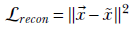
Reconstruction Loss—Just as in an autoencoder, in a properly trained VAE, the reconstruction x̃ should be close to the original input
. So, reconstruction loss is
-
KL divergence loss— In VAE, we also have a loss term proportional to the KL divergence between the distribution emitted by the encoder and the zero mean unit variance Gaussian. KL divergence measured the dissimilarity between two probability distributions and was discussed in detail in section 6.4. Here we state (following equation 6.13) that the KL divergence loss for VAE is

where q(|) denotes the latent-space map probability distribution and p() is a fixed target distribution. We want our global distribution of latent vectors to mimic the target distribution. The target is typically chosen to be a compact distribution so that the global latent vector distribution is also compact.
The popular choice for the prechosen distribution family is Gaussian and for the fixed distribution is the zero-mean unit covariance matrix Gaussian:

It should be noted that for the above choice of prior, we can evaluate the KLD loss via a closed form formula as described in section 14.7.7.
Minimizing ℒkld essentially demands that q(|) is high—that is, close to one—at the values where p() is high (see figure 14.8), because then their ratio is close to one and the logarithm is close to zero. The values of p() at the places where q(|) is low close to zero) do not matter because q(|) appears as a factor in ℒkld—the contributions to the loss by these terms are close to zero anyway.
Thus, KLD loss essentially tries to ensure that most of the sample point cloud of q(|) falls on a densely populated region of the sample point cloud of p(). Geometrically, this means the cloud of little hollow circles with black borders has a lot of overlapping mass with the target distribution. If every training data point is like that, the overall global cloud of latent vectors will also have significant overlap with the target distribution. Since the target distribution is typically chosen to be compact, this in turn ensures that the overall latent vector distribution (dark filled circles in figure 14.7) is compact. For instance, in the case when the target distribution is the zero-mean unit covariance matrix Gaussian 𝒩(;  , I), most of the mass of the latent vectors is contained within the unit radius ball. Without the KL divergence term, the latent vectors will spread throughout the latent space. In short, the KLD loss regularizes the latent space.
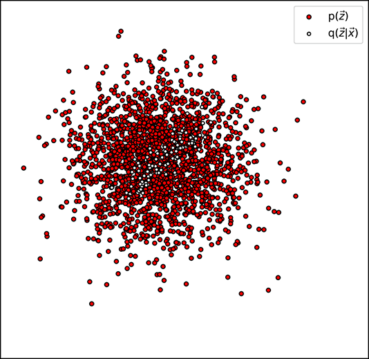
(a) Low KL divergence loss (high q(![]() |
|![]() ) coincides with high p(
) coincides with high p(![]() )
)
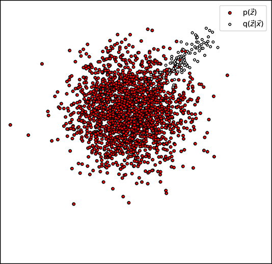
(b) High KL divergence loss (high q(![]() |
|![]() ) coincides with low p(
) coincides with low p(![]() )
)
Figure 14.8 between the encoder-generated distribution (𝒩(![]() ;
; ![]() (
(![]() ), Σ(
), Σ(![]() )) ) and the target distribution p(
)) ) and the target distribution p(![]() ) (here p(
) (here p(![]() ) ≡ 𝒩(
) ≡ 𝒩(![]() ;
; ![]() , I)) or, equivalently, low KL divergence between them.
, I)) or, equivalently, low KL divergence between them.
The encoder-decoder pair of neural networks is trained end to end to minimize the weighted sum of reconstruction loss and KLD loss. In particular, the encoder learns to emit the parameters of the q(![]() |
|![]() ) distribution.
) distribution.
During inferencing, only the encoder is used. The encoder takes an input ![]() and outputs
and outputs ![]() (
(![]() ) and Σ(
) and Σ(![]() ). We do not sample here. Instead, we use the mean directly as the latent-space representation of the input.
). We do not sample here. Instead, we use the mean directly as the latent-space representation of the input.
Notice that each input point ![]() maps to a separate Gaussian distribution q(
maps to a separate Gaussian distribution q(![]() |
|![]() = N(
= N(![]() ;
; ![]() (
(![]() ), ∑(
), ∑(![]() )). The overall distribution p(
)). The overall distribution p(![]() ) modeled by all of these together can be very complex. Yet that complexity does not affect our computation which involves only q(z|x) and p(z). This is what makes the approach powerful.
) modeled by all of these together can be very complex. Yet that complexity does not affect our computation which involves only q(z|x) and p(z). This is what makes the approach powerful.
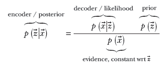
14.7.3 VAEs and Bayes’ theorem
During training, the encoder neural network stochastically maps a specific input data instance, a point ![]() in the input space, to a latent-space point
in the input space, to a latent-space point ![]() ~ 𝒩(
~ 𝒩(![]() ;
; ![]() (
(![]() ), ∑(
), ∑(![]() )). Thus the latent-space map effectively models the posterior probability p(
)). Thus the latent-space map effectively models the posterior probability p(![]() |
|![]() ). Note that we are using the symbol q(
). Note that we are using the symbol q(![]() |
|![]() ) to denote the actual distribution emitted by the encoder, while we are using the symbol p(
) to denote the actual distribution emitted by the encoder, while we are using the symbol p(![]() |
|![]() ) to denote the true (unknown) posterior probability distribution. Of course, we want these two to be as close as possible to each other: that is, we want the KL divergence between them to be minimal. Later in this section, we see how minimizing the KL divergence between q(
) to denote the true (unknown) posterior probability distribution. Of course, we want these two to be as close as possible to each other: that is, we want the KL divergence between them to be minimal. Later in this section, we see how minimizing the KL divergence between q(![]() |
|![]() ) and p(
) and p(![]() |
|![]() ) leads to the entire VAE algorithm.
) leads to the entire VAE algorithm.
The decoder maps this point (![]() ) in latent space back to the input space point x̃. As such, it models the probability distribution p(
) in latent space back to the input space point x̃. As such, it models the probability distribution p(![]() |
|![]() ).
).
The global distributions of the latent vectors ![]() effectively model p(
effectively model p(![]() ) (shown by dark-shaded filled little circles in figure 14.7). These probabilities are connected by our old friend, Bayes’ theorem:
) (shown by dark-shaded filled little circles in figure 14.7). These probabilities are connected by our old friend, Bayes’ theorem:
14.7.4 Stochastic mapping leads to latent-space smoothness
Sampling the encoder’s output from a narrow distribution is similar, but not identical, to deterministic mapping. It has a rather unexpected advantage over direct encoding. A specific input point is mapped to a slightly different point in the latent space every time it is encountered during training—all these points have to decode back to the same region in the input space. This enforces an overall smoothness over the latent space: nearby ![]() values all correspond to nearby
values all correspond to nearby ![]() values.
values.
14.7.5 Direct minimization of the posterior requires prohibitively expensive normalization
The Bayes’ theorem expression of a VAE in section 14.7.3 gives us an idea. Why not train the neural network to directly maximize the posterior probability p(![]() |
|![]() ), where X denotes the training data set? It certainly makes theoretical sense; we are choosing the latent space whose posterior probability is maximum given the training data. Of course, we must optimize one batch at a time, as we always do with neural networks.
), where X denotes the training data set? It certainly makes theoretical sense; we are choosing the latent space whose posterior probability is maximum given the training data. Of course, we must optimize one batch at a time, as we always do with neural networks.
How do we evaluate the posterior probability? The formula is as follows:
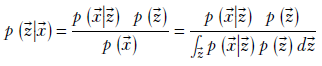
The denominator contains a sum over all values of ![]() . Remember, with every iteration, the neural network weights change, and all previously computed latent vectors become invalid. This means we have to recompute all latent vectors every iteration, which is intractable. Each iteration is 𝒪(n), and each epoch then is 𝒪(n2), where n is the number of training data instances (could be on the order of millions). We have to look for other methods. That takes us to evidence lower bound (ELBO) types of approaches.
. Remember, with every iteration, the neural network weights change, and all previously computed latent vectors become invalid. This means we have to recompute all latent vectors every iteration, which is intractable. Each iteration is 𝒪(n), and each epoch then is 𝒪(n2), where n is the number of training data instances (could be on the order of millions). We have to look for other methods. That takes us to evidence lower bound (ELBO) types of approaches.
14.7.6 ELBO and VAEs
We do not know the true probability distribution p(![]() |
|![]() ). Let’s try to learn an approximate probability distribution q(
). Let’s try to learn an approximate probability distribution q(![]() |
|![]() ) that is as close as possible to p(
) that is as close as possible to p(![]() |
|![]() ). In other words, we want to minimize the KL divergence between the two (KL divergence was introduced in section 6.4). This KL divergence is
). In other words, we want to minimize the KL divergence between the two (KL divergence was introduced in section 6.4). This KL divergence is
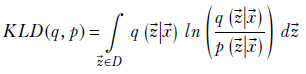
We can expand this as
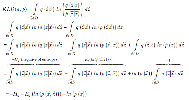
where D is the domain of ![]() : that is, the latent space, Hq is the entropy of the probability distribution (entropy was introduced in section 6.2), and Eq(ln(p(
: that is, the latent space, Hq is the entropy of the probability distribution (entropy was introduced in section 6.2), and Eq(ln(p(![]() ,
, ![]() ))) is the expected value of ln(p(
))) is the expected value of ln(p(![]() ,
, ![]() )) under the probability density q(
)) under the probability density q(![]() |
|![]() ). Rearranging terms, we get
). Rearranging terms, we get
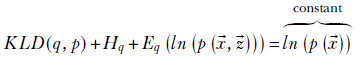
where the right-hand side is constant because it is a property of the data and cannot be adjusted during optimization. Defining the evidence lower bound (ELBO) as
ELBO = Hq + Eq(ln(p(![]() ,
, ![]() )))
)))
we get
KLD(q, p) + ELBO = constant
So, minimizing the KL divergence between p(![]() |
|![]() ) and its approximation q(
) and its approximation q(![]() |
|![]() ) is equivalent to maximizing the ELBO. We soon see that this leads to a technique for optimizing variational autoencoders.
) is equivalent to maximizing the ELBO. We soon see that this leads to a technique for optimizing variational autoencoders.
Significance of the name ELBO
Why do we call it evidence lower bound? Well, the answer is hidden in the relation KLD(q, p) + ELBO = ln(p(![]() )). The right-hand side is the evidence log-likelihood. Remember, KL divergence is always non-negative. So, the lowest value of ln(p(
)). The right-hand side is the evidence log-likelihood. Remember, KL divergence is always non-negative. So, the lowest value of ln(p(![]() )) happens when KL divergence is zero when ln(p(
)) happens when KL divergence is zero when ln(p(![]() )) = ELBO. This means the evidence log-likelihood cannot be lower than the ELBO value. Thus the ELBO is the lower bound of the evidence log-likelihood; in short, it is the evidence lower bound.
)) = ELBO. This means the evidence log-likelihood cannot be lower than the ELBO value. Thus the ELBO is the lower bound of the evidence log-likelihood; in short, it is the evidence lower bound.
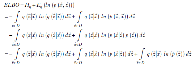
Physical significance of the ELBO
Let’s look at the physical significance of ELBO maximization:
ELBO = Hq + Eq(ln(p(![]() ,
, ![]() )))
)))
The first term is entropy. As we saw in section 6.2, this is a measure of the diffuseness of the distribution. If the points are evenly spread out in the distribution—the probability density is flat with no high peak—the entropy is high. When the distribution has few tall peaks and low values elsewhere, entropy is low (remember, for a probability density, having tall peaks implies low values elsewhere since the total volume under the function is constant: one). Thus, maximizing the ELBO means we are looking for a diffuse distribution q(![]() |
|![]() ). This, in turn, encourages smoothness in the latent space since we are effectively saying an input point
). This, in turn, encourages smoothness in the latent space since we are effectively saying an input point ![]() can map to any point around the mean
can map to any point around the mean ![]() (
(![]() ) (as emitted by the encoder) with almost equal high probability. Note that this fights a bit with the notion that each input should map to a unique point in the latent space. The solution tries to optimize between these conflicting requirements.
) (as emitted by the encoder) with almost equal high probability. Note that this fights a bit with the notion that each input should map to a unique point in the latent space. The solution tries to optimize between these conflicting requirements.
The other term—expectation of the log of joint density p(![]() ,
, ![]() ) under the probability density q(
) under the probability density q(![]() |
|![]() )—effectively measures the overlap between the two. Maximizing it is equivalent to saying q(
)—effectively measures the overlap between the two. Maximizing it is equivalent to saying q(![]() |
|![]() ) must be high where p(
) must be high where p(![]() ,
, ![]() ) is high. This seems intuitively true. The joint density p(
) is high. This seems intuitively true. The joint density p(![]() ,
, ![]() ) = p(
) = p(![]() |
|![]() )p(
)p(![]() ). It is high where both the posterior p(
). It is high where both the posterior p(![]() |
|![]() ) and prior p(
) and prior p(![]() ) are high. If q(
) are high. If q(![]() |
|![]() ) approximates the posterior, it should be high where the joint is high.
) approximates the posterior, it should be high where the joint is high.
Let’s continue to explore the ELBO. More physical significances will emerge along with an algorithm for VAE optimization:
Rearranging terms and simplifying
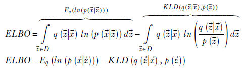
This last expression yields more physical interpretation and leads to the VAE algorithm. Let’s examine the two terms in the final ELBO expression in detail. The first term is Eq(ln(p(![]() |
|![]() ))). This is high when q(
))). This is high when q(![]() |
|![]() ) and p(
) and p(![]() |
|![]() ) are both high at the same
) are both high at the same ![]() values. For a given
values. For a given ![]() , q(
, q(![]() |
|![]() ) is high at those
) is high at those ![]() values that are likely encoder outputs (that is, latent representations) of input
values that are likely encoder outputs (that is, latent representations) of input ![]() . High p(
. High p(![]() |
|![]() ) at these same
) at these same ![]() locations implies a high probability of decoding back to the same
locations implies a high probability of decoding back to the same ![]() value from those
value from those ![]() locations. Thus, this term basically says if
locations. Thus, this term basically says if ![]() encodes to
encodes to ![]() with a high probability, then
with a high probability, then ![]() should decode back to
should decode back to ![]() with a high probability, too. Stated differently, a round trip from input to latent space back to input space should not take us far from the original input. In figure 14.7, this means the input point marked
with a high probability, too. Stated differently, a round trip from input to latent space back to input space should not take us far from the original input. In figure 14.7, this means the input point marked ![]() lies close to the output point marked
lies close to the output point marked ![]() . In other words, minimizing reconstruction loss leads to ELBO maximization.
. In other words, minimizing reconstruction loss leads to ELBO maximization.
Now consider the second term. It comes with a minus sign. Maximizing this is equivalent to minimizing the KL divergence between q(![]() |
|![]() ) and p(
) and p(![]() ). This is the regularizing term. Viewed in another way, this is the term through which we inject our belief about the basic organization of the latent space into the system. Remember that the KL divergence KLD(q(
). This is the regularizing term. Viewed in another way, this is the term through which we inject our belief about the basic organization of the latent space into the system. Remember that the KL divergence KLD(q(![]() |
|![]() ), p(
), p(![]() )) sees very little contribution from the small values of q(
)) sees very little contribution from the small values of q(![]() |
|![]() ). It is dominated by the large values of q(
). It is dominated by the large values of q(![]() |
|![]() ). In terms of figure 14.7, minimizing this KL divergence essentially ensures that most of the hollow circles fall on an area highly populated with filled circles.
). In terms of figure 14.7, minimizing this KL divergence essentially ensures that most of the hollow circles fall on an area highly populated with filled circles.
Thus, overall, maximization of ELBO is equivalent to minimizing reconstruction loss with regularization in the form of minimizing KL divergence from a specific prior distribution. This is what we do in VAEs. In every iteration, we minimize the reconstruction loss (as in ordinary AEs) and also minimize divergence from a known (or guessed) prior. Note that this does not require us to encode all training inputs per iteration. The approach is incremental—one input or input batch at a time—like any other neural network optimization. Also, although we started from finding an approximation to p(![]() |
|![]() ), the final expression does not have that anywhere. There is only the prior p(
), the final expression does not have that anywhere. There is only the prior p(![]() ) for which we can use some suitable fixed distribution.
) for which we can use some suitable fixed distribution.
14.7.7 Choice of prior: Zero-mean, unit-covariance Gaussian
The popular choice for the known prior is a zero-mean, unit-covariance matrix Gaussian, 𝒩(![]() , I) , where I is the d × d identity matrix d is the dimensionality of the latent space),
, I) , where I is the d × d identity matrix d is the dimensionality of the latent space), ![]() is d × 1 vector of all zeros. Note that minimizing the KL divergence from 𝒩(
is d × 1 vector of all zeros. Note that minimizing the KL divergence from 𝒩(![]() , I) is equivalent to restricting most of the mass within the unit ball (a hypersphere with its center at the origin and radius 1). In other words, this KL divergence term restrains the latent vectors from spreading over the ℜd and remains mostly within the unit ball. Remember that a compact set of latent vectors translates in a sense to the simplest (minimum descriptor length) representations for the input vectors: that is, a regularized latent space (section 14.6).
, I) is equivalent to restricting most of the mass within the unit ball (a hypersphere with its center at the origin and radius 1). In other words, this KL divergence term restrains the latent vectors from spreading over the ℜd and remains mostly within the unit ball. Remember that a compact set of latent vectors translates in a sense to the simplest (minimum descriptor length) representations for the input vectors: that is, a regularized latent space (section 14.6).
KL divergence from a Gaussian has a closed-form expression that we derive in section 6.4.1. We first repeat equation 6.14 for KL divergence between two Gaussians and then obtain the expression for the special case where one of the Gaussians is a zero-mean, unit-covariance Gaussian:
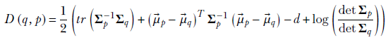
Equation 14.1
where the operator tr denotes the trace of a matrix (sum of diagonal elements) and operator det denotes the determinant. By assumption, p(![]() ) = 𝒩(
) = 𝒩(![]() , I): that is,
, I): that is, ![]() p =
p = ![]() and Σp = I. Thus,
and Σp = I. Thus,
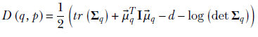
At this point, we introduce another simplifying assumption: that the covariance matrix Σq is a diagonal matrix. This means the matrix can be expressed compactly as
Σq = ![]() q
q
where ![]() q contains the elements of the main diagonal and we are not redundantly expressing the zeros in the off-diagonal elements. Note that this is not an outlandish assumption to make. We are approximating p(
q contains the elements of the main diagonal and we are not redundantly expressing the zeros in the off-diagonal elements. Note that this is not an outlandish assumption to make. We are approximating p(![]() |
|![]() ) with a Gaussian q(
) with a Gaussian q(![]() |
|![]() ) whose axes are uncorrelated.
) whose axes are uncorrelated.
Because of this assumption,
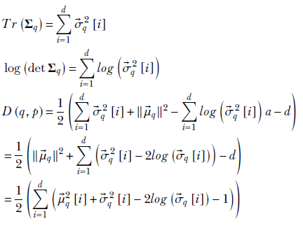
It is easy to see the expression (![]() q2[i] − 2log(
q2[i] − 2log(![]() q[i])) reaches a minimum when
q[i])) reaches a minimum when ![]() q[i] = 1. Thus, overall, KL divergence with the zero-mean, unit-covariance Gaussian is minimized when the mean is at the origin and the variances are all ones. This is equivalent to minimizing the spread of the latent vectors outside the ball of unit radius centered on the origin.
q[i] = 1. Thus, overall, KL divergence with the zero-mean, unit-covariance Gaussian is minimized when the mean is at the origin and the variances are all ones. This is equivalent to minimizing the spread of the latent vectors outside the ball of unit radius centered on the origin.
An alternative choice for the prior is a Gaussian mixture with as many components as the known number of classes. We do not discuss that here.
14.7.8 Reparameterization trick
We have avoided talking about one nasty problem so far. We said that in VAEs, the encoder emits the mean and variance of the probability density function p(![]() |
|![]() ) from which we sample the encoder output. There is a problem, however. The encoder-decoder pair are neural networks that learn via backpropagation. That is based on differentiation. Sampling is not differentiable. How do we deal with this?
) from which we sample the encoder output. There is a problem, however. The encoder-decoder pair are neural networks that learn via backpropagation. That is based on differentiation. Sampling is not differentiable. How do we deal with this?
We can use a neat trick: the so-called reparameterization trick. Let’s first explain it in the univariate case. Sampling from a Gaussian 𝒩(μ, σ) can be viewed as a combination of the following two steps:
-
Take a random sample from x from 𝒩(0,1). Note that there is no learnable parameter here; it’s a sample from a constant density function.
-
Translate the sample (add μ), and scale it (multiply by σ).
This essentially takes the sampling part out of the path for backpropagation. The encoder emits μ and σ, which are differentiable entities that we learn. Sampling is done separately from a constant density function.
The idea can be extended to a multivariate Gaussian. Sampling from 𝒩(![]() , Σ) can be broken down into sampling from 𝒩(
, Σ) can be broken down into sampling from 𝒩(![]() , I) and scaling the vector by multiplying by the matrix Σ and translating by
, I) and scaling the vector by multiplying by the matrix Σ and translating by ![]() . Thus, we have a multivariate encoder that can learn via backpropagation.
. Thus, we have a multivariate encoder that can learn via backpropagation.
NOTE Fully functional code for VAEs, executable via Jupyter Notebook, can be found at http://mng.bz/5QYD.
Listing 14.5 PyTorch- Reparameterization trick
def reparameterize(mu, log_var):
        std = torch.exp(0.5 * log_var) ①


        eps = torch.randn_like(std)    ②

        return mu + eps * std          ③
① Converts the log variance to the standard deviation
② Samples from 𝒩(![]() , I)
, I)
③ Scales by multiplying by Σ and translates by ![]()
Listing 14.6 PyTorch- VAE
from torch import nn
nz = 10
input_image_size = (1, 32, 32)            ①
conv_encoder = nn.Sequential(
            nn.Conv2d(in_channels, 32, kernel_size=3, stride=1, padding=1),
            nn.BatchNorm2d(32),
            nn.ReLU(),
            nn.MaxPool2d(kernel_size=2),  ②
            nn.Conv2d(32, 128, kernel_size=3, stride=1, padding=1),
            nn.BatchNorm2d(128),
            nn.ReLU(),
            nn.MaxPool2d(kernel_size=2),  ③
            nn.Conv2d(128, 256, kernel_size=3, stride=1, padding=1),
            nn.BatchNorm2d(256),
            nn.ReLU(),
            nn.MaxPool2d(kernel_size=2),  ④

            nn.Flatten()                  ⑤
        )
mu_fc = nn.Linear(4096, nz)               ⑥
logvar_fc = nn.Linear(4096, nz)           ⑦
① Input image size in (c, h, w) format
② Reduces to a (32, 16, 16)-sized tensor
③ Reduces to a (128, 8, 8)-sized tensor
④ Reduces to a (256, 4, 4)-sized tensor
⑤ Flattens to a 4096-sized tensor
⑥ Reduces a 4096-sized tensor to an nz-sized μ tensor
⑦ Reduces a 4096-sized tensor to an nz-sized log(σ2) tensor
Listing 14.7 PyTorch- VAE decoder
from torch import nn
decoder = nn.Sequential(
            nn.ConvTranspose2d(self.nz, out_channels=256,
             kernel_size=4, stride=1,
             padding=0, bias=False),            ①
            nn.BatchNorm2d(256),
            nn.ReLU(True),
            nn.ConvTranspose2d(256, 128, kernel_size=2,
              stride=2, padding=0, bias=False), ②
            nn.BatchNorm2d(128),
            nn.ReLU(True),
            nn.ConvTranspose2d(128, 32, kernel_size=2,
              stride=2, padding=0, bias=False), ③
            nn.BatchNorm2d(32),
            nn.ReLU(True),
            nn.ConvTranspose2d(32, in_channels, kernel_size=2,
              stride=2, padding=0, bias=False), ④
            nn.Sigmoid()
        )
① Converts (nz, 1, 1) to a (256, 4, 4)-sized tensor
② Increases to a 128, 8, 8)-sized tensor
③ Increases to a 32, 16, 16)-sized tensor
④ Increases to a 1, 32, 32)-sized tensor
Listing 14.8 PyTorch- VAE loss
recon_loss = F.binary_cross_entropy(Xr, X,
                     reduction="sum")                     ①

kld_loss = -0.5 * torch.sum(1 + log_var
                             - mu.pow(2) - log_var.exp()) ②

total_loss = recon_loss + beta * kld_loss                 ③
① Binary cross-entropy loss
② KLD(q(![]() |
|![]() ), p(
), p(![]() )) where
)) where ![]() ~ 𝒩(
~ 𝒩(![]() , I)
, I)
③ Computes the total loss
Listing 14.9 PyTorch- VAE training
conv_out = conv_encoder(X)                ①

mu = mu_fc(conv_out)                      ②
log_var = logvar_fc(conv_out)             ③

z = reparameterize(mu, log_var)           ④

Xr = self.decoder(z)                      ⑤

total_loss = recon_loss + beta * kld_loss ⑥
① Passes the input image through the convolutional encoder
② Computes μ, an nz-dimensional tensor
③ Computes log(σ2), an nz-dimensional tensor
④ Samples z via the reparameterization trick
⑤ Reconstructs the image using z via the decoder
⑥ Computes the total loss
Autoencoders vs. VAEs
Let’s revisit the familiar MNIST digits data set. It contains a training set of 60,000 images and a test set of 10,000 images. Each image is 28 × 28 in size and contains a center crop of a single digit.
Earlier, we used this data set for classification. Here, we use it an unsupervised manner: we ignore the labels during training/testing. We train both the autoencoder and the VAE end to end on this data set and look at the results (see figures 14.9 and 14.10).
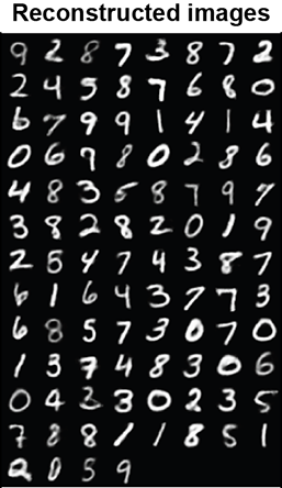
(a) Autoencoder- reconstructed images
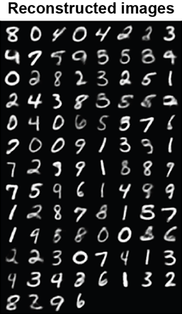
(b) VAE-reconstructed images
Figure 14.9 Comparing the reconstructed images on the test set for the autoencoder and VAE trained end to end. On a autoencoder and VAE do a pretty good job of reconstructing images from the test set.
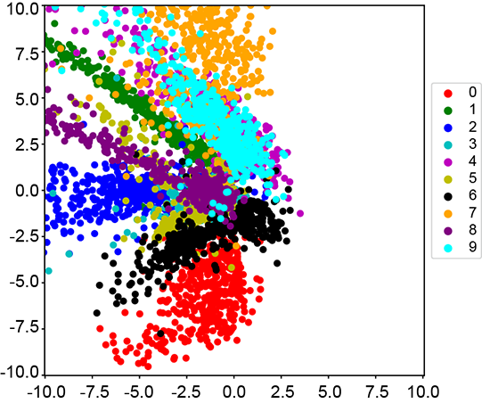
(a) Autoencoder latent space nz=2)
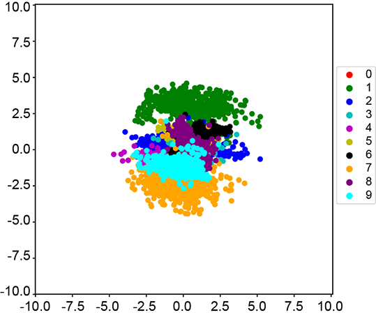
(b) VAE latent space (nz=2)
Figure 14.10 The difference between the learned latent spaces of the autoencoder and VAE. We train an autoencoder and a VAE with nz = 2 on MNIST and plot the latent space for the test set. Autoencoders only minimize the reconstruction loss, so any latent space is equally acceptable as long as the reconstruction loss is low. As expected, the learned latent space is sparse and has a very high spread. VAEs, in contrast, minimize reconstruction loss with regularization. This is done by minimizing the KL divergence between the learned latent space and a known prior distribution 𝒩(![]() , I). Adding this regularization term ensures that the latent space is constrained within a unit ball. This can be seen in figure 14.10b, where the learned latent space is much more compact.
, I). Adding this regularization term ensures that the latent space is constrained within a unit ball. This can be seen in figure 14.10b, where the learned latent space is much more compact.
The autoencoder is trained to minimize the MSE between the input image and the reconstructed image. There is no other restriction on the latent space.
The VAE is trained to maximize the ELBO. As we saw in the previous section, we can maximize the ELBO by minimizing the reconstruction loss with regularization in the form of minimizing KL divergence from a specific prior distribution: 𝒩(![]() , I) in the case of VAE. So the network is incentivized to ensure that the latent space learned is constrained within the unit ball.
, I) in the case of VAE. So the network is incentivized to ensure that the latent space learned is constrained within the unit ball.
One minor implementation detail to note is that we use binary cross-entropy instead of MSE when training VAEs. In practice, this leads to better convergence.
Summary
-
In latent-space modeling, we map input data points onto a lower-dimensional latent space. The latent space is typically a manifold consisting of points that have a property of interest in common. The property of interest can be membership to a specific class, such as all paragraphs written by Shakespeare. The latent vectors are simpler, more compact representations of the input data in which only information related to the property of interest is retained and other information is eliminated.
-
In latent space modeling, all training data input satisfies the property of interest. For instance, we can train a latent space model on paragraphs written by Shakespeare. Then the learned manifold contains points corresponding to various Shakespeare like paragraphs. Points far away from the manifold are less Shakespeare-like. By inspecting this distance, we can estimate the probability of a paragraph being written by Shakespeare. By sampling the probability distribution, we may even be able to emit pseudo-Shakespeare paragraphs.
-
Geometrically speaking, we project the input point onto the manifold. PCA performs a special form of latent space modeling where the manifold is a best-fit hyperplane for the training data.
-
Autoencoders can perform a much more powerful dimensionality reduction than PCA. An autoencoder consists of an encoder E), which maps the input data point into the lower-dimensional space, and a decoder (D), which maps the lower-dimensional representation back into the input space. It is trained to minimize the reconstruction loss: that is, the distance between the input and reconstructed (encoded, then decoded) vectors.
-
Variational autoencoders (VAEs) model latent spaces as probability distributions to impose additional constraints (over and above reconstruction loss) so that we can generate more regularized latent spaces.
-
In VAEs, the encoder maps the input to a latent representation via a stochastic process (rather than a deterministic one). It emits p(
|) as opposed to directly emitting . is obtained by sampling p(|). The decoder maps a point in latent space back to the input space. It is also modeled as a probability distribution p(|). -
The latent space learned by a VAE is much more compact and smoother (and hence more desirable) than that learned by an autoencoder.
-