Appendix
A.1 Dot product and cosine of the angle between two vectors
In section 2.5.6.1, we stated that the component of a vector ![]() along another vector
along another vector ![]() is
is ![]() ⋅
⋅ ![]() =
= ![]() T
T![]() . This is equivalent to ||
. This is equivalent to ||![]() || ||
|| ||![]() ||cos(θ), where θ is the angle between the vectors
||cos(θ), where θ is the angle between the vectors ![]() and
and ![]() .
.
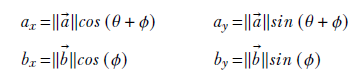
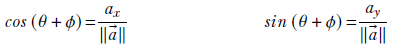
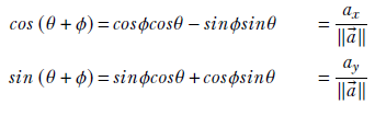
In this section, we offer a proof of this for the two-dimensional case to deepen your intuition about the geometry of dot products. From figure A.2, we can see that
which can be rewritten as
Equation A.1
Equation A.2
Using well-known trigonometric identities in equation A.1, we get
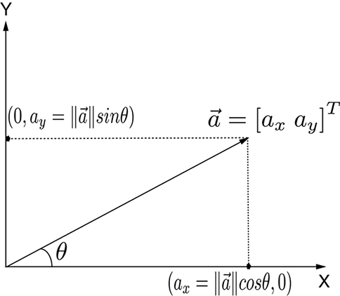
(a) Components of a 2D vector along coordinate axes. Note that ||![]() || is the length of hypotenuse.
|| is the length of hypotenuse.
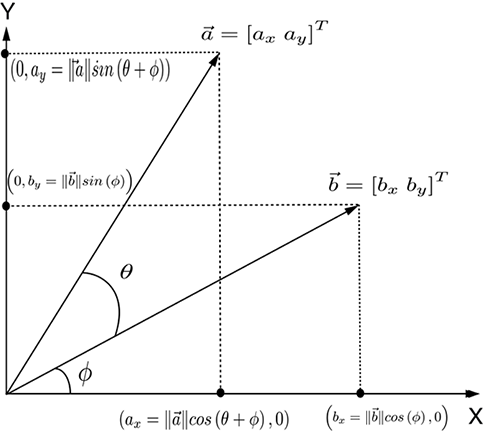
(b) Dot product as a component of one vector along another ![]() ⋅
⋅ ![]() =
= ![]() T
T![]() = axbx + ayby = ||
= axbx + ayby = ||![]() || ||
|| ||![]() ||cos(θ).
||cos(θ).
Figure A.1 Vector components and dot product
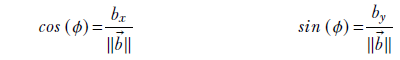
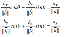
Substituting for cosϕ and sinϕ from equation A.2, we have a system of simultaneous linear equations with cosθ and sinθ as unknowns:
This system of simultaneous linear equations can be compactly written in matrix-vector form
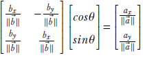
which can be simplified to
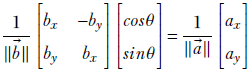
This equation can be solved to yield
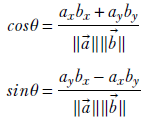
So, ||![]() || ||
|| ||![]() ||cosθ = axbx + ayby, which was to be proved.
||cosθ = axbx + ayby, which was to be proved.
A.2 Determinants
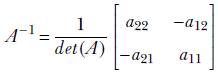
Determinant computation is tedious and numerically unstable if done naively. You should never compute one by hand—all linear algebra software packages provide routines to do this. Hence we only describe the algorithm to compute the determinant of a 2 × 2 matrix. This determinant can be computed as
det(A) = a11a22 − a12a21
The inverse is
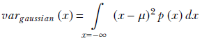
A.3 Computing the variance of a Gaussian distribution
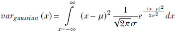
From the integral form of equation 5.13, we have
Substituting equation 5.22,
![]()
in that, we get
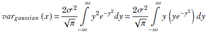
Substituting ![]() , which implies
, which implies ![]() and 2σ2y2 = (x − μ)2, we get
and 2σ2y2 = (x − μ)2, we get
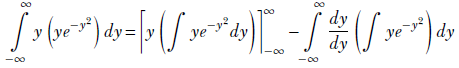
Using integration by parts,
Now, substituting v = y2, which implies dv/2 = y dy,
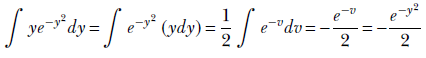
Hence,
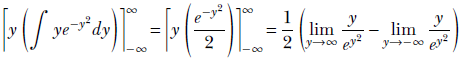
Such limits can be evaluated using L’Hospital’s rule:
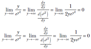
In both cases, the limit is zero because ey2 goes to positive infinity regardless of whether y goes to positive or negative infinity. Hence the denominator goes to infinity in both cases, causing the fraction to go to zero.
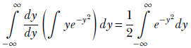
Thus the first term in the computation of vargaussian(x) becomes
![]() .
.
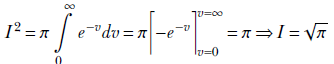
The second term
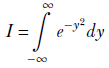
This last integral is a special one. To evaluate it, we need to go from one to two dimensions—this may be one of the very few cases where making a problem more complex helps. It is worth examining, so let’s look at it. Let
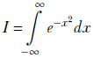
Since the variable of integration does not matter, we can also write
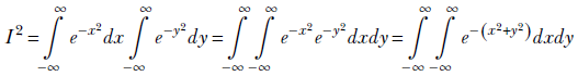
Let’s multiply them together:
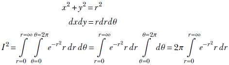
This double integral’s domain (aka region of integration) is the infinite XY plane, where x and y both range from −∞ to ∞. This same plane can also be viewed as an infinite-radius circle (an infinite-radius circle is the same as a rectangle with infinite-length sides!). Consequently, we can switch to polar coordinates, using the transformation
x = r cos(θ)
y = r cos(θ)
which implies
Substituting v = r2, which implies dv = 2rdr, we get
Thus, the second term of vargaussian(x) evaluates to ![]() . We have already shown that the first term evaluates to zero. So, we get
. We have already shown that the first term evaluates to zero. So, we get
vargaussian(x) = σ2
Thus the σ in the probability density function ![]() is the standard deviation (square root of the variance), and the μ is the expected value.
is the standard deviation (square root of the variance), and the μ is the expected value.
A.4 Two theorems in statistics
In this section, we study two important inequalities in multivariate statistics: Jensen’s inequality and the log-sum inequality.
A.4.1 Jensen’s Inequality
Consider a random variable X. For now, let’s think of these as discrete variables, although the results we will come up with apply equally well to continuous variables. Thus, let the random variable take the discrete values ![]() 1,
1, ![]() 2, ⋯,
2, ⋯, ![]() n, with probabilities p(
n, with probabilities p(![]() 1), p(
1), p(![]() 2), ⋯, p(
2), ⋯, p(![]() n).
n).
Now suppose g(![]() ) is a convex function whose domain includes these random variables. From equation 3.11, section 3.7, we know that given any convex function g(
) is a convex function whose domain includes these random variables. From equation 3.11, section 3.7, we know that given any convex function g(![]() ), for an arbitrary set of its input values
), for an arbitrary set of its input values ![]() i, i = 1⋯n and a set of weights αi i = 1⋯n satisfying
i, i = 1⋯n and a set of weights αi i = 1⋯n satisfying ![]() , the weighted sum of the function outputs is greater than or equal to the function’s output on the weighted sum of inputs: that is,
, the weighted sum of the function outputs is greater than or equal to the function’s output on the weighted sum of inputs: that is, ![]()
In particular, let’s choose the set of all random variables as input values and their probabilities as weights (αi = p(![]() i)). We can do this because probabilities sum to 1, exactly as weights are supposed to do. This leads to
i)). We can do this because probabilities sum to 1, exactly as weights are supposed to do. This leads to
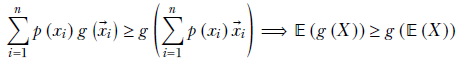
Equation A.3
Equation A.3 is Jensen’s inequality. A good mnemonic for it is: for a convex function, the expected value of the function is greater than or equal to the function of expected value. It holds for continuous random variables, too.
A.4.2 Log sum inequality
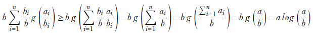
Suppose we have two sets of positive numbers a1, a2, ⋯, an and b1, b2, ⋯, bn. Let a = Σin= 1 ai and b = Σin= 1 bi. Given these, the log sum inequality theorem says,
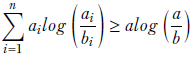
Equation A.4
To see why this is true, let’s carve out an informal proof. First let’s define g(x) = xlogx. This is a convex function because

Now, with that definition of g,
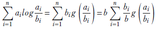
This last expression is a weighted sum of convex function outputs with the weights summing to 1 (since Σin= 1 bi/b = 1). So, we can use equation 3.11, section 3.7. Then we get
A.5 Gamma functions and distribution
To understand the gamma distribution, we need to understand the basic gamma function. First let’s do an overview of the gamma function.
A.5.1 Gamma function
The gamma function is in some sense a generalization of the factorial. The factorial function is only defined for integers and is characterized by the basic equation
n! = n(n − 1)!
The gamma function is defined by
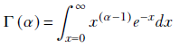
Equation A.5
Applying integration by parts to equation A.5, we get
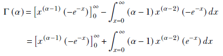
The first term is zero. This is because
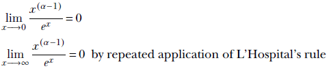
Hence,
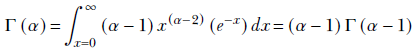
Thus, for integer values α = n, Γ(n) = n!. There are other equivalent definitions of the gamma function, but we will not discuss them here. Instead, let’s talk about the gamma distribution.
A.5.2 Gamma distribution
The probability density function for a random variable having a gamma distribution is a function with two parameters α and β:
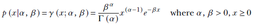
Equation A.6
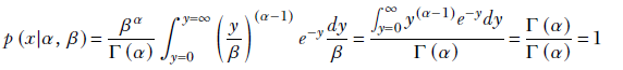
It is not hard to see that this is a proper probability density function:
![]()
By substituting y = βx, we get
If α = 1, the gamma distribution reduces to
![]()
which is graphed in figure A.2a at several values of β. The gamma distribution has two terms xα−1 and e−βx that have somewhat opposite effects: the former increases with x, while the latter deceases with x. At smaller values of x, the former wins, and the product increases with x. But eventually, the exponential starts winning and pulls the product downward asymptotically toward zero. Thus the gamma distribution has a peak. Larger β results in taller peaks and a sharper decline toward zero. Larger α moves the peak further to the right. The expected value is 𝔼(x) = α/β, as illustrated in figure A.2.
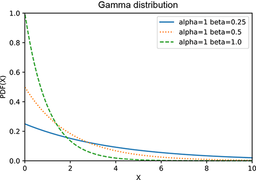
(a) Gamma distribution: α = 1, various βs
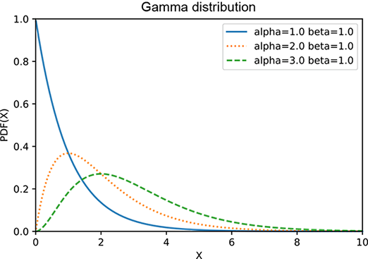
(b) Gamma distribution: β = 1, various αs
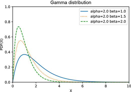
(c) Gamma distribution: α = 2, various βs
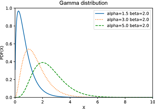
(d) Gamma distribution: β = 2, various αs
Figure A.2 Graph of a gamma distribution for various values of α and β. Larger β results in taller peaks and a sharper decline toward zero. Larger α moves the peak to the right. The expected value is 𝔼(x) = α/β.
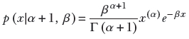
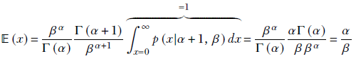
The expected value of the gamma distribution 𝔼(x) = α/β. This can be proved using a little trick so cool that it is worth discussing for that reason alone:

But the gamma distribution
or
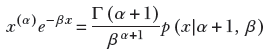
Using this,
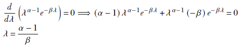
Maximum of a gamma distribution
To maximize the gamma probability density function p(λ|X) = λ(αn − 1)e−βnλ for a random variable λ, we take the derivative and equate to zero: