2 Vectors, matrices, and tensors in machine learning
This chapter covers
- Vectors and matrices and their role in datascience
- Working with eigenvalues and eigenvectors
- Finding the axes of a hyper-ellipse
At its core, machine learning, and indeed all computer software, is about number crunching. We input a set of numbers into the machine and get back a different set of numbers as output. However, this cannot be done randomly. It is important to organize these numbers appropriately and group them into meaningful objects that go into and come out of the machine. This is where vectors and matrices come in. These are concepts that mathematicians have been using for centuries—we are simply reusing them in machine learning.
In this chapter, we will study vectors and matrices, primarily from a machine learning point of view. Starting from the basics, we will quickly graduate to advanced concepts, restricting ourselves to topics relevant to machine learning.
We provide Jupyter Notebook-based Python implementations for most of the concepts discussed in this and other chapters. Complete, fully functional code that can be downloaded and executed (after installing Python and Jupyter Notebook) can be found at http://mng.bz/KMQ4. The code relevant to this chapter can be found at http://mng.bz/d4nz.
2.1 Vectors and their role in machine learning
Let’s revisit the machine learning model for a cat brain introduced in section 1.3. It takes two numbers as input, representing the hardness and sharpness of the object in front of the cat. The cat brain processes the input and generates an output threat score that leads to a decision to run away or ignore or approach and purr. The two input numbers usually appear together, and it will be handy to group them into a single object. This object will be an ordered sequence of two numbers, the first representing hardness and the second representing sharpness. Such an object is a perfect example of a vector.
Thus, a vector can be thought of as an ordered sequence of two or more numbers, also known as an array of numbers.1 Vectors constitute a compact way of denoting a set of numbers that together represent some entity. In this book, vectors are represented by lowercase letters with an overhead arrow and arrays by square brackets. For instance, the input to the cat brain model in section 1.3 was a vector  , where x0 represented hardness and x1 represented sharpness.
Outputs to machine learning models are also often represented as vectors. For instance, consider an object recognition model that takes an image as input and emits a set of numbers indicating the probabilities that the image contains a dog, human, or cat, respectively. The output of such a model is a three element vector 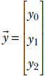 , where the number y0 denotes the probability that the image contains a dog, y1 denotes the probability that the image contains a human, and y2 denotes the probability that the image contains a cat. Figure 2.1 shows some possible input images and corresponding output vectors.
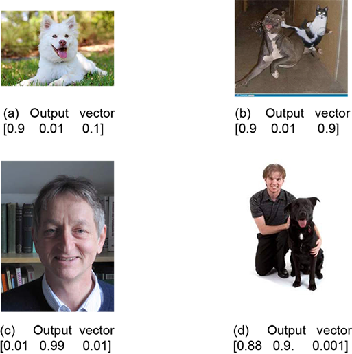
Figure 2.1 Input images and corresponding output vectors denoting probabilities that the image contains a dog and/or human and/or cat, respectively. Example output vectors are shown.
In multilayered machines like neural networks, the input and output to a layer can be vectors. We also typically represent the parameters of the model function (see section 1.3) as vectors. This is illustrated in section 2.3.
Table 2.1 Toy documents and corresponding feature vectors describing them. Words eligible for the feature vector are bold. The first element of the feature vector indicates the number of occurrences of the word gun and the second violence.
|
Docid |
Document |
Feature vector |
|---|---|---|
|
d0 |
Roses are lovely. Nobody hates roses. |
[0 0] |
|
d1 |
Gun violence has reached an epidemic proportion in America. |
[1 1] |
|
d2 |
The issue of gun violence is really over-hyped. One can find many instances of violence, where no guns were involved. |
[2 2] |
|
d3 |
Guns are for violence prone people. Violence begets guns. Guns beget violence. |
[3 3] |
|
d4 |
I like guns but I hate violence. I have never been involved in violence. But I own many guns. Gun violence is incomprehensible to me. I do believe gun owners are the most anti violence people on the planet. He who never uses a gun will be prone to senseless violence. |
[5 5] |
|
d5 |
Guns were used in a armed robbery in San Francisco last night. |
[1 0] |
|
d6 |
Acts of violence usually involves a weapon. |
[0 1] |
One particularly significant notion in machine learning and data science is the idea of a feature vector. This is essentially a vector that describes various properties of the object being dealt with in a particular machine learning problem. We will illustrate the idea with an example from the world of natural language processing (NLP). Suppose we have a set of documents. We want to create a document retrieval system where, given a new document, we have to retrieve similar documents in the system. This essentially boils down to estimating the similarity between documents in a quantitative fashion. We will study this problem in detail later, but for now, we want to note that the most natural way to approach this is to create feature vectors for each document that quantitatively describe the document. In section 2.5.6, we will see how to measure the similarity between these vectors; here, let’s focus on simply creating descriptor vectors for the documents. A popular way to do this is to choose a set of interesting words (we typically exclude words like “and,” “if,” and “to” that are present in all documents from this list), count the number of occurrences of those interesting words in each document, and make a vector of those values. Table 2.1 shows a toy example with six documents and corresponding feature vectors. For simplicity, we have considered only two of the possible set of words: gun and violence, plural or singular, uppercase or lowercase.
As a different example, the sequence of pixels in an image can also be viewed as a feature vector. Neural networks in computer vision tasks usually expect this feature vector.
2.1.1 The geometric view of vectors and its significance in machine learning
Vectors can also be viewed geometrically. The simplest example is a two-element vector ![]() . Its two elements can be taken to be x and y, Cartesian coordinates in a two-dimensional space, in which case the vector corresponds to a point in that space. Vectors with n elements represent points in an n-dimensional space. The ability to see inputs and outputs of a machine learning model as points allows us to view the model itself as a geometric transformation that maps input points to output points in some high-dimensional space. We have already seen this in section 1.4. It is an enormously powerful concept we will use throughout the book.
. Its two elements can be taken to be x and y, Cartesian coordinates in a two-dimensional space, in which case the vector corresponds to a point in that space. Vectors with n elements represent points in an n-dimensional space. The ability to see inputs and outputs of a machine learning model as points allows us to view the model itself as a geometric transformation that maps input points to output points in some high-dimensional space. We have already seen this in section 1.4. It is an enormously powerful concept we will use throughout the book.
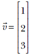
A vector represents a point in space. Also, an array of coordinate values like ![]() describes the position of one point in a given coordinate system. Hence, an array (of coordinate values) can be viewed as the quantitative representation of a vector. See figure 2.2 to get an intuitive understanding of this.
describes the position of one point in a given coordinate system. Hence, an array (of coordinate values) can be viewed as the quantitative representation of a vector. See figure 2.2 to get an intuitive understanding of this.
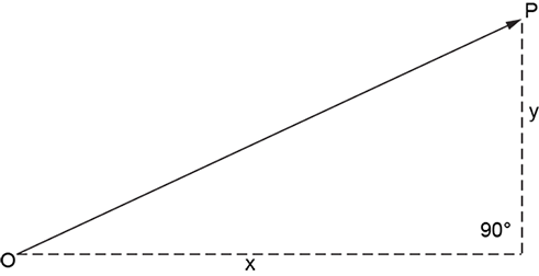
Figure 2.2 A vector describing the position of point P with respect to point O. The basic mental picture is an arrowed line. This agrees with the definition of a vector that you may have learned in high school: a vector has a magnitude (length of the arrowed line) and direction (indicated by the arrow). On a plane, this is equivalent to the ordered pair of numbers x, y, where the geometric interpretations of x and y are as shown in the figure. In this context, it is worthwhile to note that only the relative positions of the points O and P matter. If both the points are moved, keeping their relationship intact, the vector does not change.
For a real life example, consider the plane of a page of this book. Suppose we want to reach the top-right corner point of the page from the bottom-left corner. Let’s call the bottom-left corner O and the top-right corner P. We can travel the width (8.5 inches) to the right to reach the bottom-left corner and then travel the height (11 inches) upward to reach the top-right corner. Thus, if we choose a coordinate system with the bottom-left corner as the origin and the X-axis along the width, and the Y-axis along the height, point P corresponds to the array representation ![]() . But we could also travel along the diagonal from the bottom-left to the top-right corner to reach P from O. Either way, we end up at the same point P.
. But we could also travel along the diagonal from the bottom-left to the top-right corner to reach P from O. Either way, we end up at the same point P.
This leads to a conundrum. The vector ![]() represents the abstract geometric notion “position of P with respect to O” independent of our choice of coordinate axes. On the other hand, the array representation depends on the choice of a coordinate system. For example, the array
represents the abstract geometric notion “position of P with respect to O” independent of our choice of coordinate axes. On the other hand, the array representation depends on the choice of a coordinate system. For example, the array ![]() represents the top-right corner point P only under a specific choice of coordinate axes (parallel to the sides of the page) and a reference point (bottom-left corner). Ideally, to be unambiguous, we should specify the coordinate system along with the array representation. Why don’t we ever do this in machine learning? Because in machine learning, it doesn’t exactly matter what the coordinate system is as long as we stick to any fixed coordinate system. Machine learning is about minimizing loss functions (which we will study later). As such, absolute positions of point are immaterial, only relative positions matter.
represents the top-right corner point P only under a specific choice of coordinate axes (parallel to the sides of the page) and a reference point (bottom-left corner). Ideally, to be unambiguous, we should specify the coordinate system along with the array representation. Why don’t we ever do this in machine learning? Because in machine learning, it doesn’t exactly matter what the coordinate system is as long as we stick to any fixed coordinate system. Machine learning is about minimizing loss functions (which we will study later). As such, absolute positions of point are immaterial, only relative positions matter.
There are explicit rules (which we will study later) that state how the vector transforms when the coordinate system changes. We will invoke them when necessary. All vectors used in a machine learning computation must consistently use the same coordinate system or be transformed appropriately.
One other point: planar spaces, such as the plane of the paper on which this book is written, are two-dimensional (2D). The mechanical world we live in is three-dimensional (3D). Human imagination usually fails to see higher dimensions. In machine learning and data science, we often talk of spaces with thousands of dimensions. You may not be able to see those spaces in your mind, but that is not a crippling limitation. You can use 3D analogues in your head. They work in a surprisingly large variety of cases. However, it is important to bear in mind that this is not always true. Some examples where the lower-dimensional intuitions fail at higher dimensions will be shown later.
2.2 PyTorch code for vector manipulations
PyTorch is an open source machine learning library developed by Facebook’s artificial intelligence group. It is one of the most elegant practical tools for developing deep learning applications at present. In this book, we aim to familiarize you with PyTorch and similar programming paradigms alongside the relevant mathematics. Knowledge of Python basics will be assumed. You are strongly encouraged to try out all the code snippets in this book (after installing the appropriate packages like PyTorch, that is).
All the Python code in this book is produced via Jupyter Notebook. A summary of the theoretical material presented in the code is provided before the code snippet.
2.2.1 PyTorch code for the introduction to vectors
Listing 2.1 shows how to create and access vectors and subvectors and slice and dice vectors using PyTorch.
NOTE Fully functional code demonstrating how to create a vector and access its elements, executable via Jupyter Notebook, can be found at http://mng.bz/xm8q.
Listing 2.1 Introduction to vectors via PyTorch
v = torch.tensor([0.11, 0.01, 0.98, 0.12, 0.98,  ①
                ,0.85, 0.03, 0.55, 0.49, 0.99,
                0.02, 0.31, 0.55, 0.87, 0.63],
                dtype=torch.float64)             ②

first_element = v[0]
third_element = v[2]                             ③

last_element = v[-1]
second_last_element = v[-2]                      ④

second_to_fifth_elements = v[1:4]                ⑤

first_to_third_elements = v[:2]
last_two_elements = v[-2:]                       ⑥

num_elements_in_v = len(v)

u = np.array([0.11, 0.01, 0.98, 0.12, 0.98, 0.85, 0.03,
              0.55, 0.49, 0.99, 0.02, 0.31, 0.55, 0.87,
              0.63])

u = torch.from_numpy(u)                          ⑦

diff = v.sub(u)                                  ⑧

u1 = u.numpy()                                   ⑨
① torch.tensor represents a multidimensional array. The vector is a 1D tensor that can be initialized by directly specifying values.
② Tensor elements are floats by default. We can force tensors to be other types such as float64 (double).
③ The square bracket operator lets us access individual vector elements.
④ Negative indices count from the end of the array. –1 denotes the last element. -2 denotes the second-to-last element.
⑤ The colon operator slices off a range of elements from the vector.
⑥ Nothing before a colon denotes the beginning of~the~array. Nothing after a colon denotes the end~of~the array.
⑦ Torch tensors can be initialized from NumPy arrays.
⑧ The difference between the Torch tensor and its NumPy version is zero.
⑨ Torch tensors can be converted to NumPy arrays.
2.3 Matrices and their role in machine learning
Sometimes it is not sufficient to group a set of numbers into a vector. We have to collect several vectors into another group. For instance, consider the input to training a machine learning model. Here we have several input instances, each consisting of a sequence of numbers. As seen in section 2.1, the sequence of numbers belonging to a single input instance can be grouped into a vector. How do we represent the entire collection of input instances? This is where the concept of matrices comes in handy from the world of mathematics. A matrix can be viewed as a rectangular array of numbers arranged in a fixed count of rows and columns. Each row of a matrix is a vector, and so is each column. Thus a matrix can be thought of as a collection of row vectors. It can also be viewed as a collection of column vectors. We can represent the entire set of numbers that constitute the training input to a machine learning model as a matrix, with each row vector corresponding to a single training instance.
Consider our familiar cat-brain problem again. As stated earlier, a single input instance to the machine is a vector ![]() , where x0 describes the hardness of the object in front of the cat. Now consider a training dataset with many such input instances, each with a known output threat score. You might recall from section 1.1 that the goal in machine learning is to create a function that maps these inputs to their respective outputs with as little overall error as possible. Our training data may look as shown in table 2.2 (note that in real-life problems, the training dataset is usually large—often millions of input-output pairs—but in this toy problem, we will have 8 training data instances).
, where x0 describes the hardness of the object in front of the cat. Now consider a training dataset with many such input instances, each with a known output threat score. You might recall from section 1.1 that the goal in machine learning is to create a function that maps these inputs to their respective outputs with as little overall error as possible. Our training data may look as shown in table 2.2 (note that in real-life problems, the training dataset is usually large—often millions of input-output pairs—but in this toy problem, we will have 8 training data instances).
Table 2.2 Example training dataset for our toy machine learning–based cat brain
|
Input value: Hardness |
Input value: Sharpness |
Output: Threat score |
|
|---|---|---|---|
|
0 |
0.11 |
0.09 |
−0.8 |
|
1 |
0.01 |
0.02 |
−0.97 |
|
2 |
0.98 |
0.91 |
0.89 |
|
3 |
0.12 |
0.21 |
−0.68 |
|
4 |
0.98 |
0.99 |
0.95 |
|
5 |
0.85 |
0.87 |
0.74 |
|
6 |
0.03 |
0.14 |
−0.88 |
|
7 |
0.55 |
0.45 |
0.00 |
From table 2.2, we can collect the columns corresponding to hardness and sharpness into a matrix, as shown in equation 2.1—this is a compact representation of the training dataset for this problem. 2
Equation 2.1
Each row of matrix X is a particular input instance. Different rows represent different input instances. On the other hand, different columns represent different feature elements. For example, the 0th row of matrix X is the vector [x00 x01] representing the 0th input instance. Its elements, x00 and x01 represent different feature elements, hardness and sharpness respectively of the 0th training input instance.
2.3.1 Matrix representation of digital images
Digital images are also often represented as matrices. Here, each element represents the brightness at a specific pixel position (x, y coordinate) of the image. Typically, the brightness value is normalized to an integer in the range 0 to 255. 0 is black, 255 is white, and 128 is gray.3 Following is an example of a tiny image, 9 pixels wide and 4 pixels high:
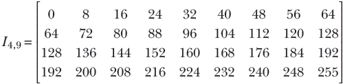
Equation 2.2
The brightness increases gradually from left to right and also from top to bottom. I00 represents the top-left pixel, which is black. I3, 8 represents the bottom-right pixel, which is white. The intermediate pixels are various shades of gray between black and white. The actual image is shown in figure 2.2.

Figure 2.3 Image corresponding to matrix I4, 9 in equation 2.2
2.4 Python code: Introducing matrices, tensors, and images via PyTorch
For programming purposes, you can think of tensors as multidimensional arrays. Scalars are zero-dimensional tensors. Vectors are one-dimensional tensors. Matrices are two-dimensional tensors. RGB images are three-dimensional tensors (colorchannels × height × width). A batch of 64 images is a four-dimensional tensor (64 × colorchannels × height × width).
Listing 2.2 Introducing matrices via PyTorch
X = torch.tensor(                                      ①
     [
        [0.11, 0.09], [0.01, 0.02], [0.98, 0.91],
        [0.12, 0.21], [0.98, 0.99], [0.85, 0.87],
        [0.03, 0.14], [0.55, 0.45]                     ②
     ]
 )

print("Shape of the matrix is: {}".format(X.shape))    ③

first_element = X[0, 0]                                ④

row_0 = X[0, :]                                        ⑤
row_1 = X[1, 0:2]                                      ⑥

column_0 = X[:, 0]                                     ⑦
column_1 = X[:, 1]                                     ⑧
① A matrix is a 2D array of numbers: i.e., a 2D tensor. The entire training data input set for a machine-learning model can be viewed as a matrix. Each input instance is one row. Row count ≡ number of training examples, column count ≡ training instance size
② Cat-brain training data input: 8 examples, each with two values (hardness, sharpness). An 8 × 2 tensor is created by specifying values.
③ The shape of a tensor is a list. For a matrix, the first list element is num rows; the second list element is num columns.
④ Square brackets extract individual matrix elements.
⑤ A standalone colon operator denotes all possible indices.
⑥ The colon operator denotes the range of indices.
⑦ 0th column
⑧ 1st column
Listing 2.3 Slicing and dicing matrices
first_3_training_examples = X[:3, ]               ①
                                                  ②
print("Sharpness of 5-7 training examples is: {}"
       .format(X[5:8, 1]))                        ③
① Ranges of rows and columns can be specified via the colon operator to slice off (extract) submatrices.
② Extracts the first three training examples (rows)
③ Extracts the sharpness feature for the 5th to 7th training examples
Listing 2.4 Tensors and images in PyTorch
tensor = torch.rand((5, 5, 3))                                  ①
                                                                ②
I49 = torch.tensor([[0, 8, 16, 24, 32, 40, 48,  56,  64],       ③
               [64,   72,  80,  88,  96, 104, 112, 120, 128],
                [128, 136, 144, 152, 160, 168, 176, 184, 192],
                [192, 200, 208, 216, 224, 232, 240, 248, 255]],
               )                                                ④

img = torch.tensor(cv2.imread('../../Figures/dog3.jpg'))        ⑤
img_b = img[:, :, 0]                                            ⑥
img_g = img[:, :, 1]                                            ⑥
img_r = img[:, :, 2]                                            ⑥
img_cropped = img[0:100, 0:100, :]                              ⑦
① PyTorch tensors can be used to represent tensors. A vector is a 1-tensor, a matrix is a 2-tensor, and a scalar is a 0-tensor.
② Creates a random tensor of specified dimensions
③ All images are tensors. An RGB image of height H, width W is a 3-tensor of shape [3, H, W].
④ 4 × 9 single-channel image shown in figure 2.3
⑤ Reads a 199 × 256 × 3 image from disk
⑥ Usual slicing dicing operators work. Extracts the red, green, and blue channels of the image as shown in figure 2.4.
⑦ Crops out a 100 × 100 subimage as shown in figure 2.5
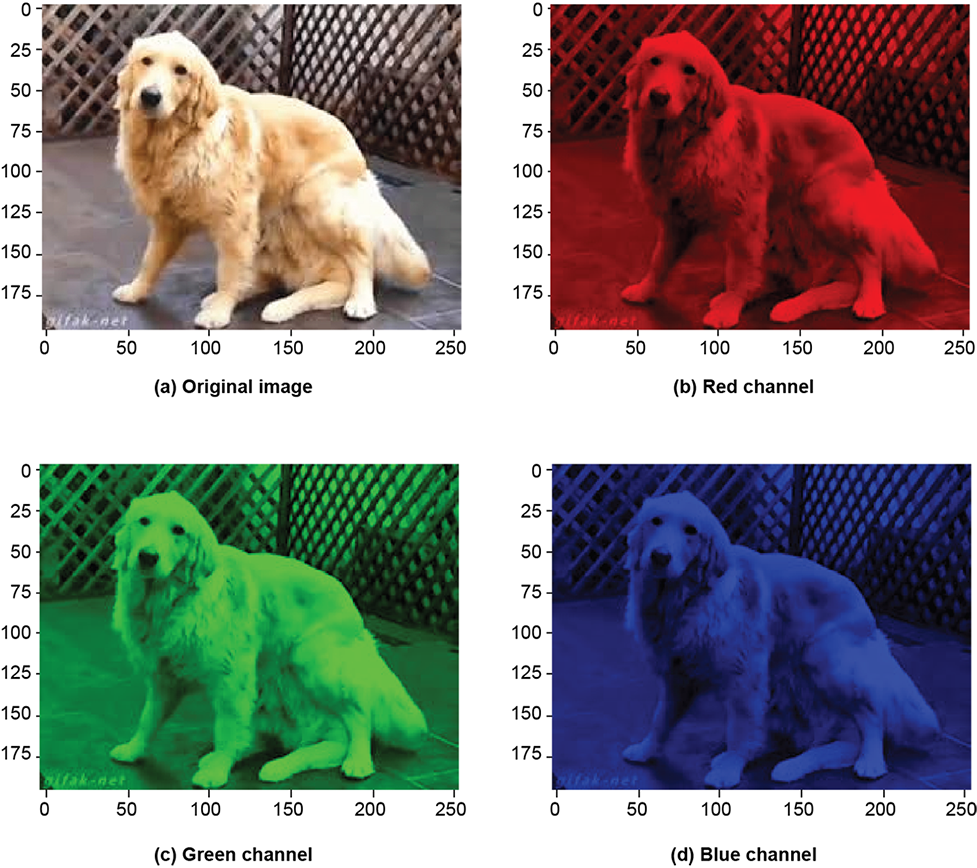
Figure 2.4 Tensors and images in PyTorch
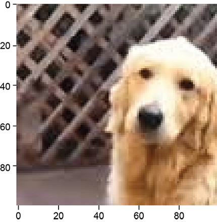
Figure 2.5 Cropped image of dog
2.5 Basic vector and matrix operations in machine learning
In this section, we introduce several basic vector and matrix operations along with examples to demonstrate their significance in image processing, computer vision, and machine learning. It is meant to be an application-centric introduction to linear algebra. But it is not meant to be a comprehensive review of matrix and vector operations, for which you are referred to a textbook on linear algebra.

Figure 2.6 Image corresponding to the transpose of matrix I4, 9 shown in equation 2.3. This is equivalent to rotating the image by 90°.
2.5.1 Matrix and vector transpose
In equation 2.2, we encountered the matrix I4, 9 depicting a tiny image. Suppose we want to rotate the image by 90° so it looks like figure 2.5. The original matrix I4, 9 and its transpose I4,T9 = I9, 4 are shown here:
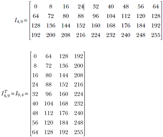
Equation 2.3
By comparing equation 2.2 and equation 2.3, you can easily see that one can be obtained from the other by interchanging the row and column indices. This operation is generally known as matrix transposition.
Formally, the transpose of a matrix Am, n with m rows and n columns is another matrix with n rows and m columns. This transposed matrix, denoted An,Tm, is such that AT[i, j] = A[j, i]. For instance, the value at row 0 column 6 in matrix I4, 9 is 48; in the transposed matrix, the same value appears in row 6 and column 0. In matrix parlance, I4, 9[0,6] = I9,T4[6,0] = 48.
Vector transposition is a special case of matrix transposition (since all vectors are matrices—a column vector with n elements is an n × 1 matrix). For instance, an arbitrary vector and its transpose are shown next:
Equation 2.4
![]()
Equation 2.5
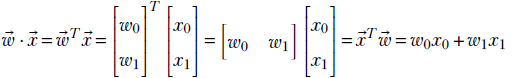
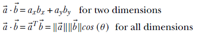
2.5.2 Dot product of two vectors and its role in machine learning
In section 1.3, we saw the simplest of machine learning models where the output is generated by taking a weighted sum of the inputs (and then adding a constant bias value). This model/machine is characterized by the weights w0, w1, and bias b. Take the rows of table 2.2. For example, for row 0, the input values are the hardness of the approaching object = 0.11 and softness = 0.09. The corresponding model output will be y = w0 × 0.11 + w1 × 0.09 + b. In fact, the goal of training is to choose w0, w1, and b such that model outputs are as close as possible to the known outputs; that is, y = w0 × 0.11 + w1 × 0.09 + b should be as close to −0.8 as possible, y = w0 × 0.01 + w1 × 0.02 + b should be as close to −0.97 as possible, that is, in general, given an input instance ![]() , the model output is y = x0w0 + x1w1 + b.
, the model output is y = x0w0 + x1w1 + b.
We will keep returning to this model throughout the chapter. But first, let’s consider a different question. In this toy example, we have only three model parameters: two weights, w0, w1, and one bias b. Hence it is not very messy to write the model output flat out as y = x0w0 + x1w1 + b. But, with longer feature vectors (that is, more weights) it will become unwieldy. Is there a compact way to represent the model output for a specific input instance, irrespective of the size of the input?
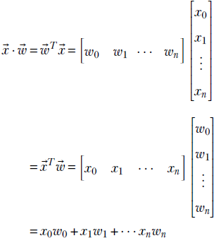
Turns out the answer is yes—we can use an operation called dot product from the world of mathematics. We have already seen in section 2.1 that an individual instance of model input can be compactly represented by a vector, say ![]() (it can have any number of input values). We can also represent the set of weights as vector
(it can have any number of input values). We can also represent the set of weights as vector ![]() —it will have the same number of items as the input vector. The dot product is simply the element-wise multiplication of the two vectors
—it will have the same number of items as the input vector. The dot product is simply the element-wise multiplication of the two vectors ![]() and
and ![]() . Formally, given two vectors and
. Formally, given two vectors and  and
and  , the dot product of the two vectors is defined as
![]()
Equation 2.6
In other words, the sum of the products of corresponding elements of the two vectors is the dot product of the two vectors, denoted ![]() ⋅
⋅ ![]() .
.
NOTE The dot product notation can compactly represent the model output as y = ![]() ⋅
⋅ ![]() + b. The representation does not increase in size even when the number of inputs and weights is large.
+ b. The representation does not increase in size even when the number of inputs and weights is large.
Consider our (by now familiar) cat-brain example again. Suppose the weight vector is  and the bias value b = 5. Then the model output for the 0th input instance from table 2.2 will be
 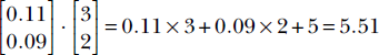 . It is another matter that these are bad choices for weight and bias parameters, since the model output 5.51 is a far cry from the desired output −0.89. We will soon see how to obtain better parameter values. For now, we just need to note that the dot product offers a neat way to represent the simple weighted sum model output.
NOTE The dot product is defined only if the vectors have the same dimensions.
Sometimes the dot product is also referred to as inner product, denoted ⟨![]() ,
, ![]() ⟩. Strictly speaking, the phrase inner product is a bit more general; it applies to infinite-dimensional vectors as well. In this book, we will often use the terms interchangeably, sacrificing mathematical rigor for enhanced understanding.
⟩. Strictly speaking, the phrase inner product is a bit more general; it applies to infinite-dimensional vectors as well. In this book, we will often use the terms interchangeably, sacrificing mathematical rigor for enhanced understanding.
2.5.3 Matrix multiplication and machine learning
Vectors are special cases of matrices. Hence, matrix-vector multiplication is a special case of matrix-matrix multiplication. We will start with that.
Matrix-vector multiplication
In section 2.5.2, we saw that given a weight vector, say ![]() , and the bias value b = 5, the weighted sum model output upon a single input instance, say
, and the bias value b = 5, the weighted sum model output upon a single input instance, say ![]() , can be represented using a vector-vector dot product
, can be represented using a vector-vector dot product ![]() . As depicted in equation 2.1, during training, we are dealing with many training data instances at the same time. In real life, we typically deal with hundreds of thousands of input instances, each having hundreds of values. Is there a way to represent the model output for the entire training dataset compactly, such that it is independent of the count of input instances and their sizes?
. As depicted in equation 2.1, during training, we are dealing with many training data instances at the same time. In real life, we typically deal with hundreds of thousands of input instances, each having hundreds of values. Is there a way to represent the model output for the entire training dataset compactly, such that it is independent of the count of input instances and their sizes?
The answer turns out to be yes. We can use the idea of matrix-vector multiplication from the world of mathematics. The product of a matrix X and column vector ![]() is another vector, denoted X
is another vector, denoted X![]() . Its elements are the dot products between the row vectors of X and the column vector
. Its elements are the dot products between the row vectors of X and the column vector ![]() . For example, given the model weight vector
. For example, given the model weight vector ![]() and the bias value b = 5, the outputs on the toy training dataset of our familiar cat-brain model (equation 2.1) can be obtained via the following steps:
and the bias value b = 5, the outputs on the toy training dataset of our familiar cat-brain model (equation 2.1) can be obtained via the following steps:
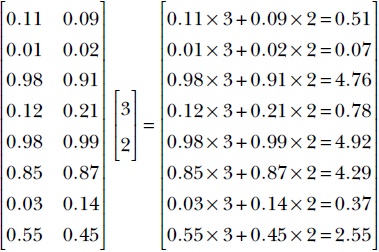
Equation 2.7
Adding the bias value of 5, the model output on the toy training dataset is
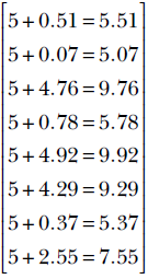
Equation 2.8
In general, the output of our simple model (biased weighted sum of input elements) can be expressed compactly as ![]() = X
= X![]() +
+ ![]() .
.
Matrix-matrix multiplication
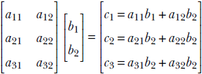
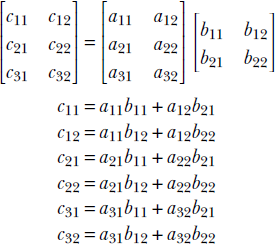
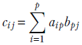
Generalizing the notion of matrix times vector, we can define matrix times matrix. A matrix with m rows and p columns, say Am, p, can be multiplied with another matrix with p rows and n columns, say Bp, n, to generate a matrix with m rows and n columns, say Cm, n: for example, Cm, n = Am, p Bp, n. Note that the number of columns in the left matrix must match the number of rows in the right matrix. Element i, j of the result matrix, Ci, j, is obtained by point-wise multiplication of the elements of the ith row vector of A and the jth column vector of B. The following example illustrates the idea:
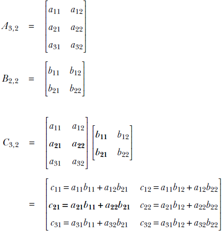
The computation for C2, 1 is shown via bolding by way of example.
NOTE Matrix multiplication is not commutative. In general, AB ≠ BA.
At this point, the astute reader may already have noted that the dot product is a special case of matrix multiplication. For instance, the dot product between two vectors ![]() and
and ![]() is equivalent to transposing either of the two vectors and then doing a matrix multiplication with the other. In other words,
is equivalent to transposing either of the two vectors and then doing a matrix multiplication with the other. In other words,
The idea works in higher dimensions, too. In general, given two vectors  and
and  , the dot product of the two vectors is defined as
Equation 2.9
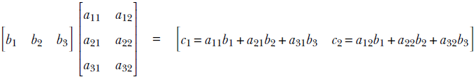
Another special case of matrix multiplication is row-vector matrix multiplication. For example, ![]() TA =
TA = ![]() or
or
Transpose of matrix products
Given two matrices A and B, where the number of columns in A matches the number of rows in B (that is, it is possible to multiply them), the transpose of the product is the product of the individual transposes, in reversed order. The rule also applies to matrix-vector multiplication. The following equations capture this rule:
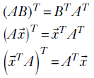
Equation 2.10
2.5.4 Length of a vector (L2 norm): Model error
Imagine that a machine learning model is supposed to output a target value ȳ, but it outputs y instead. We are interested in the error made by the model. The error is the difference between the target and the actual outputs.
Let’s apply this idea of squaring to machine learning model error. As seen earlier in section 2.5.3, given a model weight vector, say ![]() , and the bias value b = 5, the weighted sum model output upon a single input instance, say
, and the bias value b = 5, the weighted sum model output upon a single input instance, say ![]() , is
, is ![]() . The corresponding target (ideal) output, from table 2.2, is −0.8. The squared error e2 = (−0.8−5.51)2 = 39.82 gives us an idea of how good or bad the model parameters 3, 2, 5 are. For instance, if we instead use a weight vector
. The corresponding target (ideal) output, from table 2.2, is −0.8. The squared error e2 = (−0.8−5.51)2 = 39.82 gives us an idea of how good or bad the model parameters 3, 2, 5 are. For instance, if we instead use a weight vector ![]() and bias value −1, we get model output
and bias value −1, we get model output ![]() . The output is exactly the same as the target. The corresponding squared error e2 = (−0.8−(−0.8))2 = 0. This (zero error) immediately tells us that 1, 1, −1 are much better choices of model parameters than 3, 2, 5.
. The output is exactly the same as the target. The corresponding squared error e2 = (−0.8−(−0.8))2 = 0. This (zero error) immediately tells us that 1, 1, −1 are much better choices of model parameters than 3, 2, 5.
In general, the error made by a biased weighted sum model can be expressed as follows. If ![]() denotes the weight vector and
denotes the weight vector and ![]() denotes the bias, the output corresponding to an input instance
denotes the bias, the output corresponding to an input instance ![]() can be expressed as y =
can be expressed as y = ![]() ⋅
⋅ ![]() + b. Let ȳ denote the corresponding target (ground truth). Then the error is defined as e = (y−ȳ)2.
+ b. Let ȳ denote the corresponding target (ground truth). Then the error is defined as e = (y−ȳ)2.
Thus we see that we can compute the error on a single training instance by taking the difference between the model output and the ground truth and squaring it. How do we extend this concept over the entire training dataset? The set of outputs corresponding to the entire set of training inputs can be expressed as the output vector y = X![]() +
+ ![]() . The corresponding target output vector, consisting of the entire set of ground truths can be expressed as
. The corresponding target output vector, consisting of the entire set of ground truths can be expressed as ![]() . The differences between the target and model output over the entire training set can be expressed as another vector
. The differences between the target and model output over the entire training set can be expressed as another vector ![]() -
- ![]() . In our particular example:
. In our particular example:
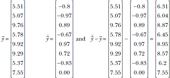
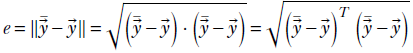
Thus the total error over the entire training dataset is obtained by taking the difference between the output and the ground truth vector, squaring its elements and adding them up. Recalling equation 2.9, this is exactly what will happen if we take the dot product of the difference vector with itself. That happens to be the definition of the squared magnitude or length or L2 norm of a vector: the dot product of the vector with itself. In the previous example, the overall training (squared) error is:
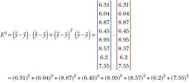
Formally, the length of a vector  , denoted ||
![]() ||, is defined as
||, is defined as ![]() . This quantity is sometimes called the L2 norm of the vector.
. This quantity is sometimes called the L2 norm of the vector.
In particular, given a machine learning model with output vector ![]() and a target vector
and a target vector ![]() , the error is the same as the magnitude or L2 norm of the difference vector
, the error is the same as the magnitude or L2 norm of the difference vector
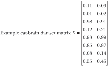
2.5.5 Geometric intuitions for vector length
For a 2D vector ![]() , as seen in figure 2.2, the L2 norm
, as seen in figure 2.2, the L2 norm ![]() is nothing but the hypotenuse of the right-angled triangle whose sides are elements of the vector. The same intuition holds in higher dimensions.
is nothing but the hypotenuse of the right-angled triangle whose sides are elements of the vector. The same intuition holds in higher dimensions.
A unit vector is a vector whose length is 1. Given any vector ![]() , the corresponding unit vector can be obtained by dividing every element by the length of that vector. For example, given
, the corresponding unit vector can be obtained by dividing every element by the length of that vector. For example, given ![]() , length
, length ![]() and the corresponding unit vector
and the corresponding unit vector  . Unit vectors typically represent a direction.
NOTE Unit vectors are conventionally depicted with the hat symbol as opposed to the little overhead arrow, as in ûTû = 1.
In machine learning, the goal of training is often to minimize the length of the error vector (the difference between the model output vector and the target ground truth vector).
2.5.6 Geometric intuitions for the dot product: Feature similarity
Consider the document retrieval problem depicted in table 2.1 one more time. We have a set of documents, each described by its own feature vector. Given a pair of such documents, we must find their similarity. This essentially boils down to estimating the similarity between two feature vectors. In this section, we will see that the dot product between a pair of vectors can be used as a measure of similarity between them.
For instance, consider the feature vectors corresponding to d5 and d6 in table 2.1. They are ![]() and
and ![]() . The dot product between them is 1 × 0 + 0 × 1 = 0. This is low and agrees with our intuition that there is no common word of interest between them, so the documents are very dissimilar. On the other hand, the dot product between feature vectors of d3 and d4 is
. The dot product between them is 1 × 0 + 0 × 1 = 0. This is low and agrees with our intuition that there is no common word of interest between them, so the documents are very dissimilar. On the other hand, the dot product between feature vectors of d3 and d4 is ![]() . This is high and agrees with our intuition that they have many commonalities in words of interest and are similar documents. Thus, we get the first glimpse of an important concept. Loosely speaking, similar vectors have larger dot products, and dissimilar vectors have near-zero dot products.
. This is high and agrees with our intuition that they have many commonalities in words of interest and are similar documents. Thus, we get the first glimpse of an important concept. Loosely speaking, similar vectors have larger dot products, and dissimilar vectors have near-zero dot products.
We will keep revisiting this problem of estimating similarity between feature vectors and solve it with more and more finesse. As a first attempt, we will now study in greater detail how dot products measure similarities between vectors. First we will show that the component of a vector along another is yielded by the dot product. Using this, we will show that the “similarity/agreement” between a pair of vectors can be estimated using the dot product between them. In particular, we will see that if the vectors point in more or less the same direction, their dot products are higher than when the vectors are perpendicular to each other. If the vectors point in opposite directions, their dot product is negative.
Dot product measures the component of one vector along another
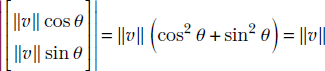
Let’s examine a special case first: the component of a vector along a coordinate axis. This can be obtained by multiplying the length of the vector with the cosine of the angle between the vector and the relevant coordinate axis. As shown for 2D in figure 2.7a, a vector ![]() can be broken into two components along the X and Y axes as
can be broken into two components along the X and Y axes as
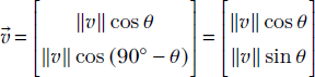
Note how the length of the vector is preserved:
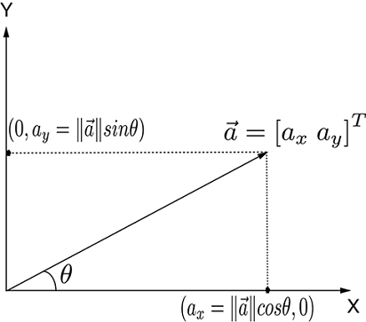
(a) Components of a 2D vector along coordinate axes. Note that ||![]() || is the length of hypotenuse.
|| is the length of hypotenuse.
(b) Dot product as a component of one vector along another ![]() ⋅
⋅ ![]() =
= ![]() T
T![]() = axbx + ayby = ||
= axbx + ayby = ||![]() || ||
|| ||![]() ||cos(θ).
||cos(θ).
Figure 2.7 Vector components and dot product
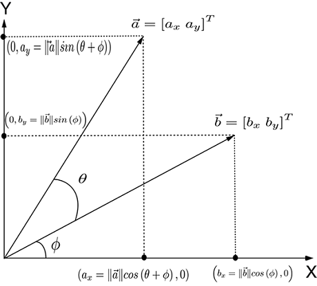
Now let’s study the more general case of the component of one vector in the direction of another arbitrary vector (figure 2.7b). The component of a vector ![]() along another vector
along another vector ![]() is
is ![]() ⋅
⋅ ![]() =
= ![]() T
T![]() . This is equivalent to ||
. This is equivalent to ||![]() || ||
|| ||![]() ||cos(θ), where θ is the angle between the vectors
||cos(θ), where θ is the angle between the vectors ![]() and
and ![]() . (This has been proven for the two-dimension case discussed in section A.1 of the appendix. You can read it if you would like deeper intuition.)
. (This has been proven for the two-dimension case discussed in section A.1 of the appendix. You can read it if you would like deeper intuition.)
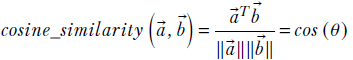
Dot product measures the agreement between two vectors
The dot product can be expressed using the cosine of the angle between the vectors. Given two vectors ![]() and
and ![]() , if θ is the angle between them, we have see figure 2.7b)
, if θ is the angle between them, we have see figure 2.7b)
Equation 2.11
Expressing the dot product using cosines makes it easier to see that it measures the agreement (aka correlation) between two vectors. If the vectors have the same direction, the angle between them is 0 and the cosine is 1, implying maximum agreement. The cosine becomes progressively smaller as the angle between the vectors increases, until the two vectors become perpendicular to each other and the cosine is zero, implying no correlation—the vectors are independent of each other. If the angle between them is 180°, the cosine is −1, implying that the vectors are anti-correlated. Thus, the dot product of two vectors is proportional to their directional agreement.
What role do the vector lengths play in all this? The dot product between two vectors is also proportional to the lengths of the vectors. This means agreement scores between bigger vectors are higher (an agreement between the US president and the German chancellor counts more than an agreement between you and me).
If you want the agreement score to be neutral to the vector length, you can use a normalized dot product between unit-length vectors along the same directions:
Dot product and the difference between two unit vectors
To obtain further insight into how the dot product indicates agreement or correlation between two directions, consider the two unit vectors  and
and  . The difference between them is
 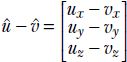 .
.
Note that since they are unit vectors, ![]() . The length of the difference vector
. The length of the difference vector
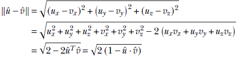
From the last equality, it is evident that a larger dot product implies a smaller difference: that is, more agreement between the vectors.
2.6 Orthogonality of vectors and its physical significance
Try moving an object at right angles to the direction in which you are pushing it. You will find it impossible. The larger the angle, the less effective your force vector becomes (finally becoming totally ineffective at a 90° angle). This is why it is easy to walk on a horizontal surface (you are moving at right angles to the direction of gravitational pull, so the gravity vector is ineffective) but harder on an upward incline (the gravity vector is having some effect against you).
These physical notions are captured mathematically in the notion of a dot product. The dot product between two vectors ![]() (say, the push vector) and
(say, the push vector) and ![]() (say, the displacement of the pushed object vector) is ||
(say, the displacement of the pushed object vector) is ||![]() || ||
|| ||![]() ||cosθ, where θ is the angle between the two vectors. When θ is 0 (the two vectors are aligned), cosθ = 1, the maximum possible value of cosθ, so push is maximally effective. As θ increases, cosθ decreases, and push becomes less and less effective. Finally, at θ = 90°, cosθ = 0, and push becomes completely ineffective.
||cosθ, where θ is the angle between the two vectors. When θ is 0 (the two vectors are aligned), cosθ = 1, the maximum possible value of cosθ, so push is maximally effective. As θ increases, cosθ decreases, and push becomes less and less effective. Finally, at θ = 90°, cosθ = 0, and push becomes completely ineffective.
Two vectors are orthogonal if their dot product is zero. Geometrically, this means the vectors are perpendicular to each other. Physically, this means the two vectors are independent: one cannot influence the other. You can say there is nothing in common between orthogonal vectors. For instance, the feature vector for d5 is ![]() and that for d6 is
and that for d6 is ![]() in table 2.1. These are orthogonal (dot product is zero), and you can easily see that none of the feature words (gun, violence) are common to both documents.
in table 2.1. These are orthogonal (dot product is zero), and you can easily see that none of the feature words (gun, violence) are common to both documents.
2.7 Python code: Basic vector and matrix operations via PyTorch
In this section, we use Python PyTorch code to illustrate many of the concepts discussed earlier.
NOTE Fully functional code for this section, executable via Jupyter Notebook, can be found at http://mng.bz/ryzE.
2.7.1 PyTorch code for a matrix transpose
The following listing shows the PyTorch code for a matrix transpose.
Listing 2.5 Transpose
I49 = torch.stack([torch.arange(0, 72, 8), torch.arange(64, 136, 8),   ①
                torch.arange(128, 200, 8), torch.arange(192, 264, 8)])

I49_t = torch.transpose(I49, 0, 1)                                     ②

for i in range(0, I49.shape[0]):
    for j in range(0, I49.shape[1]):
        assert I49[i][j] == I49_t[j][i]                                ③


assert torch.allclose(I49_t, I49.T, 1e-5)                              ④
① The torch.arange function creates a vector whose elements go from start to stop in increments of step. Here we create a 4 × 9 image corresponding to I4,9 in equation 2.2, shown in figure 2.3.
② The transpose operator interchanges rows and columns. The 4 × 9 image becomes a 9 × 4 image (see figure 2.6. The element at position (i, j) is interchanged with the element at position (j, i).
③ Interchanged elements of the original and transposed matrix are equal.
④ The .T operator retrieves the transpose of an array.
2.7.2 PyTorch code for a dot product
The dot product of two vectors ![]() and
and ![]() represents the components of one vector along the other. Consider two vectors
represents the components of one vector along the other. Consider two vectors ![]() = [a1 a2 a3] and
= [a1 a2 a3] and ![]() = [b1 b2 b3]. Then
= [b1 b2 b3]. Then ![]() .
.![]() = a1b1 + a2b2 + a3b3.
= a1b1 + a2b2 + a3b3.
Listing 2.6 Dot product
a = torch.tensor([1, 2, 3])
b = torch.tensor([4, 5, 6])
a_dot_b = torch.dot(a, b)
print("Dot product of these two vectors is: "
              "{}".format(a_dot_b))               ①

# Dot product of perpendicular vectors is zero
vx = torch.tensor([1, 0]) # a vector along X-axis
vy = torch.tensor([0, 1]) # a vector along Y-axis
print("Example dot product of orthogonal vectors:"
              " {}".format(torch.dot(vx, vy)))    ②
① Outputs 32: 1 ∗ 4 + 2 ∗ 5 + 3 ∗ 6
② Outputs 0: 1 ∗ 0 + 0 ∗ 1
2.7.3 PyTorch code for matrix vector multiplication
Consider a matrix Am, n with m rows and n columns that is multiplied with a vector ![]() n with n elements. The result is a m element column vector
n with n elements. The result is a m element column vector ![]() m . In the following example, m = 3 and n = 2.
m . In the following example, m = 3 and n = 2.
In general,
![]()
Listing 2.7 Matrix vector multiplication
X = torch.tensor([[0.11, 0.09], [0.01, 0.02], [0.98, 0.91], [0.12, 0.21], ①
              [0.98, 0.99], [0.85, 0.87], [0.03, 0.14], [0.55, 0.45],
              [0.49, 0.51], [0.99, 0.01], [0.02, 0.89], [0.31, 0.47],
              [0.55, 0.29], [0.87, 0.76], [0.63, 0.24]])                  ②

w = torch.rand((2, 1))                                                    ③
b = 5.0
  = torch.matmul(X, w) + b                                                ④
① A linear model comprises a weight vector ![]() and bias b. For each training data instance
and bias b. For each training data instance ![]() i, the model outputs yi =
i, the model outputs yi = ![]() iT
iT![]() + b. For the training data matrix X (whose rows are training data instances), the model outputs X
+ b. For the training data matrix X (whose rows are training data instances), the model outputs X![]() +
+ ![]() =
= ![]()
② Cat-brain 15 × 2 training data matrix (equation 2.7)
③ Random initialization of weight vector
④ Model training output: ![]() = X
= X![]() + b. The scalar b is automatically replicated to create a vector.
+ b. The scalar b is automatically replicated to create a vector.
2.7.4 PyTorch code for matrix-matrix multiplication
Consider a matrix Am, p with m rows and p columns. Let’s multiply it with another matrix Bp, n with p rows and n columns. The resultant matrix Cm, n contains m rows and n columns. Note that the number of columns in the left matrix A should match the number of rows in the right matrix B:
In general,
Listing 2.8 Matrix-matrix multiplication
A = torch.tensor([[1, 2], [3, 4], [5, 6]])
B = torch.tensor([[7, 8], [9, 10]])

C = torch.matmul(A, B)                              ①
                                                    ②
  w = torch.tensor([1, 2, 3])
  x = torch.tensor([4, 5, 6])
  assert torch.dot(w, x) == torch.matmul(w.T, x)    ③
① C = AB ⟹ C[i, j] is the dot product of the ith row of A and jth column of B.
② 
③ The dot product can be viewed as a row matrix multiplied by a column matrix.
2.7.5 PyTorch code for the transpose of a matrix product
Given two matrices A and B, where the number of columns in A matches the number of rows in B, the transpose of their product is the product of the individual transposes in reversed order: (AB)T = BTAT.
Listing 2.9 Transpose of a matrix product
assert torch.all(torch.matmul(A, B).T == torch.matmul(B.T, A.T))  ①

assert torch.all(torch.matmul(A.T, x).T == torch.matmul(x.T, A))  ②
① Asserts equality between (AB)T and BTAT
② Applies to matrix-vector multiplication, too: (AT![]() )T =
)T = ![]() TA
TA
2.8 Multidimensional line and plane equations and machine learning
Geometrically speaking, what does a machine learning classifier really do? We provided the outline of an answer in section 1.4. You are invited to review that and especially figures 1.2 and 1.3. We will briefly summarize here.
Inputs to a classifier are feature vectors. These vectors can be viewed as points in some multidimensional feature space. The task of classification then boils down to separating the points belonging to different classes. The points may be all jumbled up in the input space. It is the model’s job to transform them into a different (output) space where it is easier to separate the classes. A visual example of this was provided in figure 1.3.
What is the geometrical nature of the separator? In a very simple situation, such as the one depicted in figure 1.2, the separator is a line in 2D space. In real-life situations, the separator is often a line or a plane in a high-dimensional space. In more complicated situations, the separator is a curved surface, as depicted in figure 1.4.
In this section, we will study the mathematics and geometry behind two types of separators, lines, and planes in high-dimensional spaces, aka hyperlines and hyperplanes.
2.8.1 Multidimensional line equation
In high school geometry, we learned y = mx + c as the equation of a line. But this does not lend itself readily to higher dimensions. Here we will study a better representation of a straight line that works equally well for any finite-dimensional space.
As shown in figure 2.8, a line joining vectors ![]() and
and ![]() can be viewed as the set of points we will encounter if we
can be viewed as the set of points we will encounter if we
-
Start at point

-
Travel along the direction
 −
−
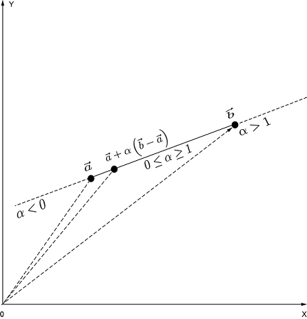
Figure 2.8 Any point ![]() on the line joining two vectors
on the line joining two vectors ![]() ,
, ![]() is given by
is given by ![]() =
= ![]() + α(
+ α(![]() −
−![]() ).
).
Different points on the line are obtained by traveling different distances. Denoting this arbitrary distance by α, the equation of the line joining vectors ![]() and
and ![]() can be expressed as
can be expressed as
Equation 2.12
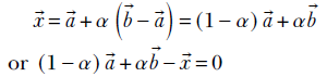
Equation 2.12 says that any point on the line joining ![]() and
and ![]() can be obtained as a weighted combination of
can be obtained as a weighted combination of ![]() and
and ![]() , the weights being α and 1 − α. By varying α, we obtain different points on the line. Also, different ranges of α values yield different segments on the line. As shown in figure 2.8, values of α between 0 and 1 yield points between
, the weights being α and 1 − α. By varying α, we obtain different points on the line. Also, different ranges of α values yield different segments on the line. As shown in figure 2.8, values of α between 0 and 1 yield points between ![]() and
and ![]() . Negative values of α yield points to the left of
. Negative values of α yield points to the left of ![]() . Values of α greater than 1 yield points to the right of
. Values of α greater than 1 yield points to the right of ![]() . This equation for a line works for any dimensions, not just two.
. This equation for a line works for any dimensions, not just two.
2.8.2 Multidimensional planes and their role in machine learning
In section 1.5, we encountered classifiers. Let’s take another look at them. Suppose we want to create a classifier that helps us make buy or no-buy decisions on stocks based on only three input variables: 1) momentum, or the rate at which the stock price is changing positive momentum means the stock price is increasing and vice versa); 2) the dividend paid last quarter; and (3) volatility, or how much the price has fluctuated in the last quarter. Let’s plot all training points in the feature space with coordinate axes corresponding to the variables momentum, dividend, volatility. Figure 2.9 shows that the classes can be separated by a plane in the three-dimensional feature space.
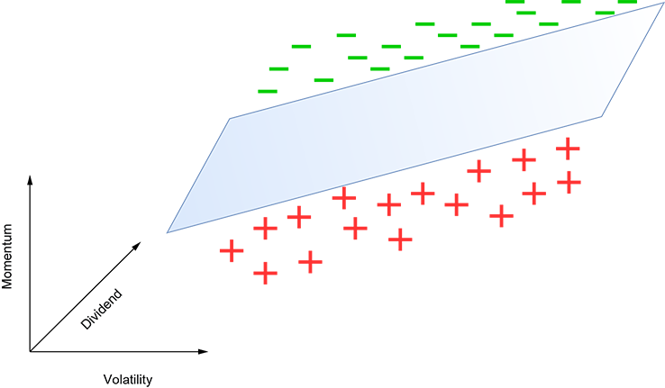
Figure 2.9 A toy machine learning classifier for stock buy vs. no-buy decision-making. A plus (+) indicates no-buy, and a dash (-) indicates buy. The decision is made based on three input variables: momentum, dividend, and volatility.
Geometrically speaking, our model simply corresponds to this plane. Input points above the plane indicate buy decisions (dashes [-]), and input points indicate no-buy decisions (pluses [+]). In general, you want to buy high-positive-momentum stocks, so points at the higher end of the momentum axis are likelier to be buy. However, this is not the only indicator. For more volatile stocks, we demand higher momentum to switch from no-buy to buy. This is why the plane slopes upward (higher momentum) as we move rightward (higher volatility). Also, we demand less momentum for stocks with higher dividends. This is why the plane slopes downward (lower momentum) as we go toward higher dividends.
Real problems have more dimensions, of course (since many more inputs are involved in the decision), and the separator becomes a hyperplane. Also, in real-life problems, the points are often too intertwined in the input space for any separator to work. We first have to apply a transformation that maps the point to an output space where it is easier to separate. Given their significance as class separators in machine learning, we will study hyperplanes in this section.
In high school 3D geometry, we learned ax + by + cz + d = 0 as the equation of a plane. Now we will study a version of it that works in higher dimensions.
Geometrically speaking, given a plane (in any dimension), we can find a direction called the normal direction, denoted n̂, such that
-
If we take any pair of points on the plane, say
 0 and , …
 -
The line joining
and 0—i.e., the vector − 0—is orthogonal to n̂.
Thus, if we know a fixed point on the plane, say ![]() 0, then all points on the plane will satisfy
0, then all points on the plane will satisfy
n̂ · (![]() −
− ![]() 0) = 0
0) = 0
or
n̂T(![]() −
− ![]() 0) = 0
0) = 0
Thus we can express the equation of a plane as
n̂T![]() − n̂T
− n̂T![]() 0 = 0
0 = 0
Equation 2.13
Equation 2.13 is depicted pictorially in figure 2.10.
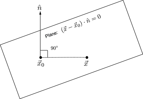
Figure 2.10 The normal to the plane is the same at all points on the plane. This is the fundamental property of a plane. n̂ depicts that normal direction. Let ![]() 0 be a point on the plane. All other points on the plane, depicted as
0 be a point on the plane. All other points on the plane, depicted as ![]() , will satisfy the equation (
, will satisfy the equation (![]() −
−![]() 0) ⋅ n̂ = 0. This physically says that the line joining a known point
0) ⋅ n̂ = 0. This physically says that the line joining a known point ![]() 0 on the plane and any other arbitrary point
0 on the plane and any other arbitrary point ![]() on the plane is at right angles to the normal n̂. This formulation works for any dimension.
on the plane is at right angles to the normal n̂. This formulation works for any dimension.
In section 1.3, equation 1.3, we encountered the simplest machine learning model: a weighted sum of inputs along with a bias. Denoting the inputs as ![]() , the weights as
, the weights as ![]() , and the bias as b, this model was depicted as
, and the bias as b, this model was depicted as
![]() T
T![]() + b = 0
+ b = 0
Equation 2.14
Comparing equations 2.13 and 2.14 , we get the geometric significance: the simple model of equation 1.3 is nothing but a planar separator. Its weight vector ![]() corresponds to the plane’s orientation (normal). The bias b corresponds to the plane’s location (a fixed point on the plane). During training, we are learning the weights and biases—this is essentially learning the orientation and position of the optimal plane that will separate the training inputs. To be consistent with the machine learning paradigm, henceforth we will write the equation of a hyperplane as equation 2.14 for some constant
corresponds to the plane’s orientation (normal). The bias b corresponds to the plane’s location (a fixed point on the plane). During training, we are learning the weights and biases—this is essentially learning the orientation and position of the optimal plane that will separate the training inputs. To be consistent with the machine learning paradigm, henceforth we will write the equation of a hyperplane as equation 2.14 for some constant ![]() and b.
and b.
Note that ![]() need not be a unit-length vector. Since the right-hand side is zero, if necessary, we can divide both sides by ||
need not be a unit-length vector. Since the right-hand side is zero, if necessary, we can divide both sides by ||![]() || to convert to a form like equation 2.13.
|| to convert to a form like equation 2.13.
The sign of the expression ![]() T
T![]() + b has special significance. All points
+ b has special significance. All points ![]() for which
for which ![]() T
T![]() + b < 0 lie on the same side of the hyperplane. All points
+ b < 0 lie on the same side of the hyperplane. All points ![]() for which
for which ![]() T
T![]() + b > 0 lie on the other side of the hyperplane. And of course, all points
+ b > 0 lie on the other side of the hyperplane. And of course, all points ![]() for which
for which ![]() T
T![]() + b = 0 lie on the hyperplane.
+ b = 0 lie on the hyperplane.
It should be noted that the 3D equation ax + by + cz + d = 0 is a special case of equation 2.14 because ax + by + cz + d = 0 can be rewritten as
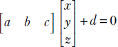
which is same as ![]() T
T![]() + b = 0 with
+ b = 0 with  and
and  . Incidentally, this tells us that in 3D, the normal to the plane ax + by + cz + d = 0 is
 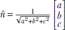 .
.
2.9 Linear combinations, vector spans, basis vectors, and collinearity preservation
by now, it should be clear that machine learning and data science are all about points in high-dimensional spaces. Consequently, it behooves us to have a decent understanding of these spaces. For instance, given a space, we may need to ask, “Would it be possible to express all points in the space in terms of a set of a few vectors? What is the smallest set of vectors we really need for that purpose?” This section is devoted to the study of these questions.
2.9.1 Linear dependence
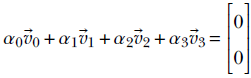
Consider the vectors (points) shown in figure 2.11. The corresponding vectors in 2D are
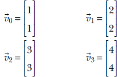
We can find four scalars α0 = 2, α1 = 2, α2 = 2, and α3 = −3 such that
If we can find such scalars, not all zero, we say the vectors ![]() 0,
0, ![]() 1,
1, ![]() 2, and
2, and ![]() 3 are linearly dependent. The geometric picture to keep in mind is that points corresponding to linearly dependent vectors lie on a single straight line in the space containing them.
3 are linearly dependent. The geometric picture to keep in mind is that points corresponding to linearly dependent vectors lie on a single straight line in the space containing them.
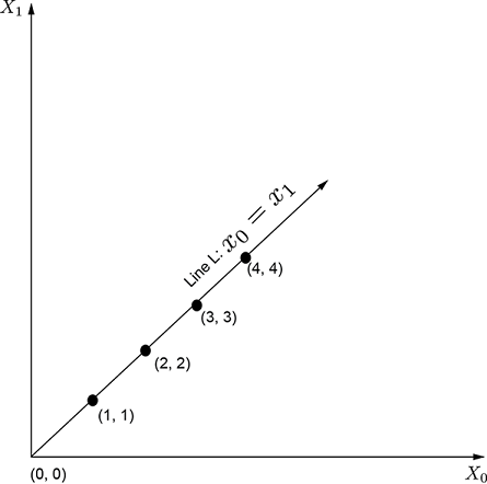
Figure 2.11 Linearly dependent points in a 2D plane
Collinearity implies linear dependence
Proof: Let ![]() ,
, ![]() and
and ![]() be three collinear vectors. From equation 2.12, there exists some α ∈ ℝ such that
be three collinear vectors. From equation 2.12, there exists some α ∈ ℝ such that
![]() = (1−α)
= (1−α)![]() + α
+ α![]()
This equation can be rewritten as
α1![]() + α2
+ α2![]() + α3
+ α3![]() = 0
= 0
where α1 = (1−α), α2 = α and α3 = −1. Thus we have proven that three collinear vectors ![]() ,
, ![]() , and
, and ![]() must also be linearly dependent.
must also be linearly dependent.
Linear combination
Given a set of vectors ![]() 1,
1, ![]() 2, ….
2, …. ![]() n and a set of scalar weights α1, α2, …αn, the weighted sum α1
n and a set of scalar weights α1, α2, …αn, the weighted sum α1![]() 1 + α2
1 + α2![]() 2 + + … αn
2 + + … αn![]() n is called a linear combination.
n is called a linear combination.
Generic multidimensional definition of linear dependence
A set of vectors ![]() 1,
1, ![]() 2, ….
2, …. ![]() n are linearly dependent if there exists a set of weights α1, α2, …αn, not all zeros, such that α1
n are linearly dependent if there exists a set of weights α1, α2, …αn, not all zeros, such that α1![]() 1 + α2
1 + α2![]() 2 + + … αn
2 + + … αn![]() n = 0. For example, the row vectors [1 1] and [2 2] are linearly dependent, since –2[1 1] + [2 2] = 0.
n = 0. For example, the row vectors [1 1] and [2 2] are linearly dependent, since –2[1 1] + [2 2] = 0.
2.9.2 Span of a set of vectors
Given a set of vectors ![]() 1,
1, ![]() 2, ….
2, …. ![]() n, their span is defined as the set of all vectors that are linear combinations of the original set . This includes the original vectors.
n, their span is defined as the set of all vectors that are linear combinations of the original set . This includes the original vectors.
For example, consider the two vectors ![]() and
and ![]() . The span of these two vectors is the entire plane containing the two vectors. Any vector, for instance, the vector
. The span of these two vectors is the entire plane containing the two vectors. Any vector, for instance, the vector ![]() can be expressed as a weighted sum 18
can be expressed as a weighted sum 18![]() x⊥ + 97
x⊥ + 97![]() y⊥.
y⊥.
You can probably recognize that ![]() and
and ![]() are the familiar Cartesian coordinate axes (X-axis and Y-axis, respectively) in the 2D plane.
are the familiar Cartesian coordinate axes (X-axis and Y-axis, respectively) in the 2D plane.
2.9.3 Vector spaces, basis vectors, and closure
We have been talking informally about vector spaces. It is time to define them more precisely.
Vector spaces
A set of vectors (points) in n dimensions form a vector space if and only if the operations of addition and scalar multiplication are defined on the set. In particular, this implies that it is possible to take linear combinations of members of a vector space.
Basis vectors
Given a vector space, a set of vectors that span the space is called a basis for the space. For instance, for the space ℝ2, the two vectors ![]() and
and ![]() are basis vectors. This essentially means any vector in ℝ2 can be expressed as a linear combination of these two. The notion can be extended to higher dimensions. For ℝn, the vectors
are basis vectors. This essentially means any vector in ℝ2 can be expressed as a linear combination of these two. The notion can be extended to higher dimensions. For ℝn, the vectors 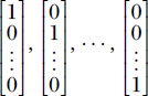 form a basis.
The alert reader has probably guessed by now that the basis vectors are related to coordinate axes. In fact, the basis vectors just described constitute the Cartesian coordinate axes.
So far, we have only seen examples of basis vectors that are mutually orthogonal, such as the dot product of the two basis vectors in ℝ2 shown earlier: 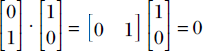 . However, basis vectors do not have to be orthogonal. Any pair of linearly independent vectors forms a basis in ℝ2. Basis vectors, then, are by no means unique. That said, orthogonal vectors are most convenient, as we shall see later.
Minimal and complete basis
Exactly n vectors are needed to span a space with dimensionality n. This means the basis set for a space will have at least as many elements as the dimensionality of the space. That many basis vectors are also sufficient to form a basis. For instance, exactly n vectors are needed to form a basis in (that is, span) ℝn.
A related fact is that in ℝn, any set of m vectors with m > n will be linearly dependent. In other words, the largest size of a set of linearly independent vectors in an n-dimensional space is n.
Closure
A set of vectors is said to be closed under linear combination if and only if the linear combination of any pair of vectors in the set also belongs to the same set. Consider the set of points ℝ2. Recall that this is the set of vectors with two real elements. Take any pair of vectors ![]() and
and ![]() in ℝ2: for instance,
in ℝ2: for instance, ![]() and
and ![]() . Any linear combination of these two vectors will also comprise two real numbers—that is, will belong to ℝ2. We say ℝ2 is a vector space since it is closed under linear combination.
. Any linear combination of these two vectors will also comprise two real numbers—that is, will belong to ℝ2. We say ℝ2 is a vector space since it is closed under linear combination.
Consider the space ℝ2. Geometrically speaking, this represents a two dimensional plane. Let’s take two points on this plane, ![]() and
and ![]() . Linear combinations of
. Linear combinations of ![]() ,
, ![]() geometrically correspond to points on the line joining them. We know that if two points lie on a plane, the entire line will also lie on the plane. Thus, in two dimensions, a plane is closed under linear combinations. This is the geometrical intuition behind the notion of closure on vector spaces. It can be extended to arbitrary dimensions.
geometrically correspond to points on the line joining them. We know that if two points lie on a plane, the entire line will also lie on the plane. Thus, in two dimensions, a plane is closed under linear combinations. This is the geometrical intuition behind the notion of closure on vector spaces. It can be extended to arbitrary dimensions.
On the other hand, the set of points on the surface of a sphere is not closed under linear combination because the line joining an arbitrary pair of points on this set will not wholly lie on the surface of that sphere.
2.10 Linear transforms: Geometric and algebraic interpretations
Inputs to a machine learning or data science system are typically feature vectors (introduced in section 2.1) in high-dimensional spaces. Each individual dimension of the feature vector corresponds to a particular property of the input. Thus, the feature vector is a descriptor for the particular input instance. It can be viewed as a point in the feature space. We usually transform the points to a friendlier space where it is easier to perform the analysis we are trying to do. For instance, if we are building a classifier, we try to transform the input into a space where the points belonging to different classes are more segregated (see section 1.3 in general and figure 1.3 in particular for simple examples). Sometimes we transform to simplify the data, eliminating axes along which there is scant variation in the data. Given their significance in machine learning, in this section we will study the basics of transforms.
Informally, a transform is an operation that maps a set of points vectors) to another. Given a set S of n × 1 vectors, any m × n matrix T can be viewed as a transform. If ![]() belongs to the set S, multiplication with the matrix T will map (transform)
belongs to the set S, multiplication with the matrix T will map (transform) ![]() to a vector T
to a vector T![]() . We will later see that matrix multiplication is a subclass of transforms that preserve collinearity—points that lie on a straight line before the transformation will continue to lie on a (possibly different) straight line post the transformation. For instance, consider the matrix
. We will later see that matrix multiplication is a subclass of transforms that preserve collinearity—points that lie on a straight line before the transformation will continue to lie on a (possibly different) straight line post the transformation. For instance, consider the matrix
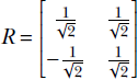
In section 2.14, we will see that this is a special kind of matrix called a rotation matrix; for now, simply consider it an example of a matrix. R is a transformation operator that maps a point in a 2D plane to another point in the same plane. In mathematical notation, R : ℝ2 → ℝ2. In fact, as depicted in figure 2.14, this transformation (multiplication by matrix R) rotates the position vector of a point in the 2D plane by an angle of 45°.
The output and input points may belong to different spaces in such transforms. For instance, consider the matrix
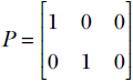
It is not hard to see that this matrix projects 3D points to the 2D X-Y plane:
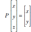
Hence, this transformation (multiplication by matrix P) projects points from three to two dimensions. In mathematical parlance, P : ℝ3 → ℝ2.
The transforms R and P share a common property: they preserve collinearity. This means a set of vectors (points) ![]() ,
, ![]() ,
, ![]() , ⋯ that originally lay on a straight line remain so after the transformation.
, ⋯ that originally lay on a straight line remain so after the transformation.
Let’s check this out for the rotation transformation in the example from section 2.9. There we saw four vectors:
These vectors all lie on a straight L : x = y. The rotation transformed versions of these vectors are
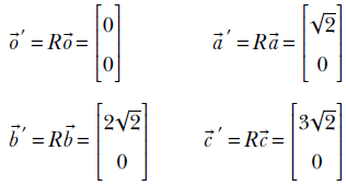
It is trivial to see that the transformed vectors also lie on a (different) straight line. In fact, ![]() ′,
′, ![]() ′,
′, ![]() ′,
′, ![]() ′ lie on the Y-axis, which is the 45° rotated version of the original line y = x.
′ lie on the Y-axis, which is the 45° rotated version of the original line y = x.
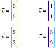
The projection transform represented by matrix P also preserves collinearity. Consider four collinear vectors in 3D:
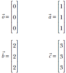
The corresponding transformed vectors
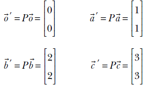
also lie on a straight line in 2D.
The class of transforms that preserves collinearity are known as linear transforms. They can always be represented as a matrix multiplication. Conversely, all matrix multiplications represent a linear transformation. A more formal definition is provided later.
2.10.1 Generic multidimensional definition of linear transforms
A function ϕ is a linear transform if and only if it satisfies
ϕ(α![]() + β
+ β![]() ) = αϕ(
) = αϕ(![]() ) + βϕ(
) + βϕ(![]() ) ∀ α, β ∈ ℝ
) ∀ α, β ∈ ℝ
Equation 2.15
In other words, a transform is linear if and only if the transform of the linear combination of two vectors is the same as the linear combination (with the same weights) of the transforms of individual vectors. (This can be remembered as: Linear transform means transforms of linear combinations are same as linear combinations of transforms.) Multiplication with a rotation or projection matrix (shown earlier) is a linear transform.
2.10.2 All matrix-vector multiplications are linear transforms
Let’s verify that matrix multiplication satisfies the definition of linear mapping (equation 2.15). Let ![]() ,
, ![]() ∈ ℝn be two arbitrary n-dimensional vectors and Am, n be an arbitrary matrix with n columns. Then following the standard rules of matrix-vector multiplication,
∈ ℝn be two arbitrary n-dimensional vectors and Am, n be an arbitrary matrix with n columns. Then following the standard rules of matrix-vector multiplication,
A(α![]() + β
+ β![]() ) = α(A
) = α(A![]() ) + β(A
) + β(A![]() )
)
which mimics equation 2.15 with ϕ replaced with matrix A. Thus we have proven that all matrix multiplications are linear transforms. The reverse is not true. In particular, linear transforms that operate on infinite-dimensional vectors are not matrices. But all linear transforms that operate on finite-dimensional vectors can be expressed as matrices. (The proof is a bit more complicated and will be skipped.)
Thus, in finite dimensions, multiplication with a matrix and linear transformation are one and the same thing. In section 2.3, we saw the array view of matrices. The corresponding geometric view, that all matrices represent linear transformation, was presented in this section.
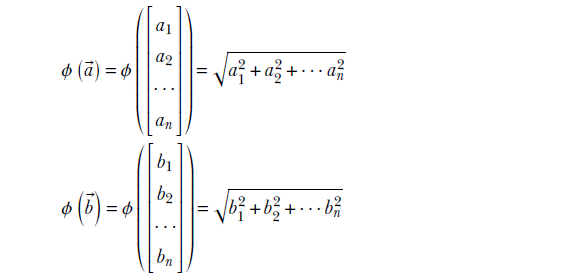
Let’s finish this section by studying an example of a transform that is not linear. Consider the function
ϕ(![]() ) = ||
) = ||![]() ||
||
for ![]() ∈ ℝn. This function ϕ maps n-dimensional vectors to a scalar that is the length of the vector, ϕ : ℝn → ℝ. We will examine if it satisfies equation 2.15 with α1 = α2 = 1. For two specific vectors
∈ ℝn. This function ϕ maps n-dimensional vectors to a scalar that is the length of the vector, ϕ : ℝn → ℝ. We will examine if it satisfies equation 2.15 with α1 = α2 = 1. For two specific vectors ![]() ,
, ![]() ∈ ℝn,
∈ ℝn,
Now
![]()
and
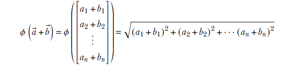
Clearly, these two are not equal; hence, we have violated equation 2.15: ϕ is a nonlinear mapping.
2.11 Multidimensional arrays, multilinear transforms, and tensors
We often hear the term tensor in connection with machine learning. Google’s famous machine learning platform is named TensorFlow. In this section, we will introduce you to the concept of a tensor.
2.11.1 Array view: Multidimensional arrays of numbers
A tensor may be viewed as a generalized n-dimensional array—although, strictly speaking, not all multidimensional arrays are tensors. We will learn more about the distinction between multidimensional arrays and tensors when we study multilinear transforms. For now, we will not worry too much about the distinction. A vector can be viewed as a 1 tensor, a matrix is a 2 tensor, and a scalar is a 0 tensor.
In section 2.3, we saw that digital images are represented as 2D arrays (matrices). A color image—where each pixel is represented by three colors, R, G, and B (red, green, and blue)—is an example of a multidimensional array or tensor. This is because it can be viewed as a combination of three images: the R, G, and B images, respectively.
The inputs and outputs to each layer in a neural network are also tensors.
2.12 Linear systems and matrix inverse
Machine learning today is usually an iterative process. Given a set of training data, you want to estimate a set of machine parameters that will yield target values (or close approximations to them) on training inputs. The number of training inputs and the size of the parameter set are often very large. This makes it impossible to have a closed-form solution where we solve for the unknown parameters in a single step. Solutions are usually iterative. We start with a guessed set of values for the parameters and iteratively improve the guess by processing training data.
Having said that, we often encounter smaller problems in real life. We are better off using more traditional closed-form techniques here since they are much faster and more accurate. This section is devoted to gaining some insights into these techniques.
Let’s go back to our familiar cat-brain problem and refer to its training data in table 2.2. As before, we are still talking about a weighted sum model with three parameters: weights w0, w1 and bias b. Let’s focus on the top three rows from the table, repeated here in table 2.2 for convenience.
Table 2.3 Example training dataset for our toy machine learning–based cat brain
|
Input value: Hardness |
Input value: Sharpness |
Output: Threat score |
|
|---|---|---|---|
|
0 |
0.11 |
0.09 |
−0.8 |
|
1 |
0.01 |
0.02 |
−0.97 |
|
2 |
0.98 |
0.91 |
0.89 |
The training data says that with a hardness value 0.11 and a sharpness value 0.09, we expect the system’s output to match or closely approximate) the target value −0.8, and so on. In other words, our estimated values for parameters w0, w1, b should ideally satisfy
0.11w0 + 0.09w1 + b = –0.8
0.01w0 + 0.02w1 + b = –0.97
0.98w0 + 0.91 w1 + b = 0.89
We can express this via matrix multiplication as the following equation:
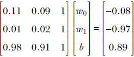
How do we obtain the values of w0, w1, b that make this equation true? That is, how do we solve this equation? There are formal methods (discussed later) to directly solve such equations for w0, w1, and b (in this very simple example, you might just “see” that w0 = 1, w1 = 1, b = −1 solves the equation, but we need a general method).
This equation is an example of a class of equations called a linear system. A linear system in n unknowns x1, x2, x3, ⋯, xn,
a11x1 + a12x2 + a13x3 + … + a1nxn = b1
a21x1 + a22x2 + a23x3 + … + a2nxn = b2
⁞
an1x1 + an2x2 + an3x3 + … + annxn = bn
can be expressed via matrix and vectors as
A![]() =
= ![]()
where
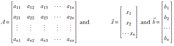
Although equivalent, the matrix depiction is more compact and dimension-independent. In machine learning, we usually have many variables (thousands), so this compactness makes a significant difference. Also, A![]() =
= ![]() looks similar to the one-variable equation we know so well: ax = b. In fact, many intuitions can be transferred from 1D to higher dimensions.
looks similar to the one-variable equation we know so well: ax = b. In fact, many intuitions can be transferred from 1D to higher dimensions.
What is the solution to the 1D equation? You may have learned it in fifth grade: The solution of ax = b is x = a−1b where a−1 = 1/a, a ≠ 0.
We can use the same notation in all dimensions. The solution of A![]() =
= ![]() is
is ![]() = A−1
= A−1![]() , where A−1 is the matrix inverse. The inverse matrix A−1 has the determinant of the matrix, 1/det(A), as a factor. We will not discuss determinant and inverse matrix computation here—you can obtain that in any standard linear algebra textbook—but will state some facts that lend insights into determinants and inverse matrices:
, where A−1 is the matrix inverse. The inverse matrix A−1 has the determinant of the matrix, 1/det(A), as a factor. We will not discuss determinant and inverse matrix computation here—you can obtain that in any standard linear algebra textbook—but will state some facts that lend insights into determinants and inverse matrices:
-
The inverse matrix A−1 is related to matrix A in the same way the scalar a−1 is related to the scalar a. a−1 exists if and only if a ≠ 0. Analogously, A−1 exists if det(A) ≠ 0, where det(A) refers to the determinant of a matrix.
-
The product of a scalar a and its inverse a−1 is 1. Analogously, AA−1 = A−1A = I, where I denotes the identity matrix that is the higher-dimension analog for 1 in scalar arithmetic. It is a matrix in which the diagonal terms are 1 and all other terms are 0. The n-dimensional identity matrix is as follows:
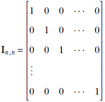
When there is no subscript, the dimensionality can be inferred from the context. For any matrix A, IA = AI = A. For any vector ![]() , I
, I![]() =
= ![]() TI =
TI = ![]() . These can be easily verified using the rules of matrix multiplication.
. These can be easily verified using the rules of matrix multiplication.
There are completely precise but tedious rules for computing determinants and matrix inverses. Despite the importance of the concept, we rarely need to compute them in life as all linear algebra software packages provide routines to do this. Furthermore, computing matrix inverses is not good programming practice because it is numerically unstable. We will not discuss the direct computation of determinant or matrix inverse here (except that in section A.2 of the appendix, we show how to compute the determinant of a 2 × 2 matrix). We will discuss pseudo-inverses, which have more significance in machine learning.
2.12.1 Linear systems with zero or near-zero determinants,and ill-conditioned systems
We saw earlier that a linear system A![]() =
= ![]() has the solution
has the solution ![]() = A−1
= A−1![]() . But A−1 has 1/det(A) as a factor. What if the determinant is zero?
. But A−1 has 1/det(A) as a factor. What if the determinant is zero?
The short answer: when the determinant is zero, the linear system cannot be exactly solved. We may still attempt to come up with an approximate answer (see section 2.12.3), but an exact solution is not possible.
Let’s examine the situation a bit more closely with the aid of an example. Consider the following system of equations:
x1 + x2 = 2
2x1 + 2x2 = 4
It can be rewritten as a linear system with a square matrix:
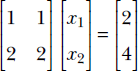
But you can quickly see that the system of equations cannot be solved. The second equation is really the same as the first. In fact, we can obtain the second by multiplying the first by a scalar, 2. Hence, we don’t really have two equations: we have only one, so the system cannot be solved. Now examine the row vectors of matrix A. They are [1 1] and [2 2]. They are linearly dependent because −2[1 1] + [2 2] = 0. Now examine the determinant of matrix A (section A.2 of the appendix shows how to compute the determinant of a 2 × 2 matrix). It is 2 × 1 − 1 × 2 = 0. These results are not coincidences. Any one of them implies the other. In fact, the following statements about the linear system A![]() =
= ![]() (with a square matrix) are equivalent:
(with a square matrix) are equivalent:
-
Matrix A has a row/column that can be expressed as a weighted sum of the others.
-
Matrix A has linearly dependent rows or columns.
-
Matrix A has zero determinant (such matrices are called singular matrices).
-
The inverse of matrix A (i.e., A−1) does not exist. A is called singular.
-
The linear system cannot be solved.
The system is trying to tell you that you have fewer equations than you think you have, and you cannot solve the system of equations.
Sometimes the determinant is not exactly zero but close to zero. Although solvable in theory, such systems are numerically unstable. Small changes in input cause the result to change drastically. For instance, consider this nearly singular matrix:
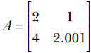
Equation 2.16
Its determinant is 0.002, close to zero. Let ![]() be a vector.
be a vector.
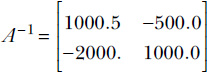
Equation 2.17
(Note how large the elements of A−1 are. This is due to division by an extremely small determinant and, in turn, causes the instability illustrated next.) The solution to the equation ![]() . But if we change
. But if we change ![]() just a little and make
just a little and make ![]() , the solution changes to a drastically different
, the solution changes to a drastically different ![]() . This is inherently unstable and arises from the near singularity of the matrix A. Such linear systems are called ill-conditioned.
. This is inherently unstable and arises from the near singularity of the matrix A. Such linear systems are called ill-conditioned.
2.12.2 PyTorch code for inverse, determinant, and singularity testing of matrices
Inverting a matrix and computing its determinant can be done with a single function call from the linear algebra package linalg.
Listing 2.10 Matrix inverse for an invertible matrix (nonzero determinant)
def determinant(A):
    return torch.linalg.det(A)

def inverse(A):
    return torch.linalg.inv(A)

A = torch.tensor([[2, 3], [2, 2]], dtype=torch.float    ①

A_inv = inverse(A)                                      ②

I = torch.eye(2)                                        ③

assert torch.all(torch.matmul(A, A_inv) == I)           ④
assert torch.all(torch.matmul(A_inv, A) == I)


assert torch.all(torch.matmul(I, A) ==  A)
assert torch.all(A == torch.matmul(A,I))                ⑤
① ![]()
② ![]()
③ The PyTorch function torch.eye(n) generates an identity matrix I of size n
④ Verify ![]()
⑤ I is like 1. Verify AI = IA = A
A singular matrix is a matrix whose determinant is zero. Such matrices are non-invertible. Linear systems of equations with singular matrices cannot be solved.
Listing 2.11 Singular matrix
B = torch.tensor([[1, 1], [2, 2]], dtype=torch.float)   ①
try:

    B_inv = inverse(B)                                  ②

except RuntimeError as e:
    print("B cannot be inverted: {}".format(B, e))
① ![]()
② Determinant = 1 × 2 − 2 × 1 = 0. Singular matrix; attempting to compute the inverse causes a runtime error.
2.12.3 Over- and under-determined linear systems in machine learning
What if the matrix A is not square? This implies that the number of equations does not match the number of unknowns. Does such a system even make sense? Surprisingly, it does. As a rule, machine learning systems fall in this category: the number of equations corresponds to the number of training data instances collected, while the number of unknowns is a function of the number of weights in the model which is a function of the particular model family chosen to represent the system. These are independent of each other. As stated earlier, we often solve these systems iteratively. Nonetheless, it is important to understand linear systems with nonsquare matrices A, to gain insight.
There are two possible cases, assuming that the matrix A is m × n (m rows and n columns):
-
Case 1: m > n (more equations than unknowns; overdetermined system)
-
Case 2: m < n (fewer equations than unknown; underdetermined system)
For instance, table 2.2 leads to an overdetermined linear system. Let’s write the system of equations:
0.11 w0 + 0.09 w1 + b = –0.8
0.01 w0 + 0.02 w1 + b = –0.97
0.98 w0 + 0.91 w1 + b = 0.89
0.12 w0 + 0.21 w1 + b = –0.68
0.98 w0 + 0.99 w1 + b = 0.95
0.85 w0 + 0.87 w1 + b = 0.74
0.03 w0 + 0.14 w1 + b = –0.88
0.55 w0 + 0.45 w1 + b = 0.00
These yield the following overdetermined linear system:
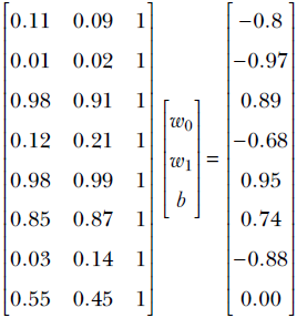
Equation 2.18
This is a nonsquare 15 × 3 linear system. There are only 3 unknowns to solve for (w0, w1, b), and there are 15 equations. This is highly redundant: we needed only three equations and could have solved it via linear system solution techniques (section 2.12). But the important thing to note is this: the equations are not fully consistent. There is no single set of values for the unknown that will satisfy all of them. In other words, the training data is noisy—an almost universal occurrence in real-life machine learning systems. Consequently, we have to find a solution that is optimal (causes as little error as possible) over all the equations.
We want to solve it such that the overall error ||A![]() −
− ![]() || is minimized. In other words, we are looking for
|| is minimized. In other words, we are looking for ![]() such that A
such that A![]() is as close to
is as close to ![]() as possible. This closed-form that is, non-iterative) method is an extremely important precursor to machine learning and data science. We will revisit this multiple times, most notably in sections 2.12.4 and 4.5.
as possible. This closed-form that is, non-iterative) method is an extremely important precursor to machine learning and data science. We will revisit this multiple times, most notably in sections 2.12.4 and 4.5.
2.12.4 Moore Penrose pseudo-inverse of a matrix
The pseudo-inverse is a handy technique to solve over- or under-determined linear systems. Suppose we have an overdetermined system with the not-necessarily square m × n matrix A:
A![]() =
= ![]()
Since A is not guaranteed to be square, we can take neither the determinant nor the inverse in general. So the usual A−1![]() does not work. At this point, we observe that although the inverse cannot be taken, transposing the matrix is always possible. Let’s multiply both sides of the equation with AT:
does not work. At this point, we observe that although the inverse cannot be taken, transposing the matrix is always possible. Let’s multiply both sides of the equation with AT:
A![]() =
= ![]() ⇔ ATA
⇔ ATA![]() = AT
= AT![]()
Notice that ATA is a square matrix: its dimensions are (m×n) × (n×m) = m × m. Let’s assume, without proof for the moment, that it is invertible. Then
A![]() =
= ![]() ⇔ ATA
⇔ ATA![]() = AT
= AT![]() ⇔
⇔ ![]() = (ATA)−1AT
= (ATA)−1AT![]()
Hmmm, not bad; we seem to be onto something. In fact, we just derived the pseudo-inverse of matrix A, denoted A + = (ATA)−1AT. Unlike the inverse, the pseudo-inverse does not need the matrix to be square with linearly independent rows. Much like the regular linear system, we get the solution of the (possibly nonsquare) system of equations as A![]() =
= ![]() ⇔
⇔ ![]() = A +
= A + ![]() .
.
The pseudo-inverse-based solution actually minimizes the error ||A![]() −
− ![]() ||. We will provide an intuitive proof of that in section 2.12.5. Meanwhile, you are encouraged to write the Python code to evaluate (ATA)−1AT
||. We will provide an intuitive proof of that in section 2.12.5. Meanwhile, you are encouraged to write the Python code to evaluate (ATA)−1AT![]() and verify that it approximately yields the expected answer
and verify that it approximately yields the expected answer ![]() for equation 2.18.
for equation 2.18.
2.12.5 Pseudo-inverse of a matrix: A beautiful geometric intuition
A matrix Am × n can be rewritten in terms of its column vectors as [![]() 1,
1, ![]() 2, …
2, … ![]() n], where
n], where ![]() 1 …
1 … ![]() n are all m-dimensional vectors. Then if
n are all m-dimensional vectors. Then if  , we get A
![]() = x1
= x1![]() 1 + x2
1 + x2![]() 2 + ⋯ xn
2 + ⋯ xn![]() n. In other words, A
n. In other words, A![]() is just a linear combination of the column vectors of A with the elements of
is just a linear combination of the column vectors of A with the elements of ![]() as the weights (you are encouraged to write out a small 3 × 3 system and verify this). The space of all vectors of the form A
as the weights (you are encouraged to write out a small 3 × 3 system and verify this). The space of all vectors of the form A![]() (that is, the linear span of the column vectors of A) is known as the column space of A.
(that is, the linear span of the column vectors of A) is known as the column space of A.
The solution to the linear system of equations A![]() =
= ![]() can be viewed as finding the
can be viewed as finding the ![]() that minimizes the difference of A
that minimizes the difference of A![]() and
and ![]() : that is, minimizes ||A
: that is, minimizes ||A![]() −
− ![]() ||. This means we are trying to find a point in the column space of A that is closest to the point
||. This means we are trying to find a point in the column space of A that is closest to the point ![]() . Note that this interpretation does not assume a square matrix A. Nor does it assume a nonzero determinant. In the friendly case where the matrix A is square and invertible, we can find a vector
. Note that this interpretation does not assume a square matrix A. Nor does it assume a nonzero determinant. In the friendly case where the matrix A is square and invertible, we can find a vector ![]() such that A
such that A![]() becomes exactly equal to
becomes exactly equal to ![]() , which makes ||A
, which makes ||A![]() −
− ![]() || = 0. If A is not square, we will try to find
|| = 0. If A is not square, we will try to find ![]() such that A
such that A![]() is closer to
is closer to ![]() than any other vector in the column space of A. Mathematically speaking, 4
than any other vector in the column space of A. Mathematically speaking, 4
![]()
Equation 2.19
From geometry, we intuitively know that the closest point to ![]() in the column space of A is obtained by dropping a perpendicular from
in the column space of A is obtained by dropping a perpendicular from ![]() to the column space of A (see figure 2.12). The point where this perpendicular meets the column space is called the projection of
to the column space of A (see figure 2.12). The point where this perpendicular meets the column space is called the projection of ![]() on the column space of A. The solution vector
on the column space of A. The solution vector ![]() to equation 2.19 that we are looking for should correspond to the projection of
to equation 2.19 that we are looking for should correspond to the projection of ![]() on the column space of A. This in turn means
on the column space of A. This in turn means ![]() − A
− A![]() is orthogonal (perpendicular) to all vectors in the column space of A (see figure 2.12). We represent arbitrary vectors in the column space of A as A
is orthogonal (perpendicular) to all vectors in the column space of A (see figure 2.12). We represent arbitrary vectors in the column space of A as A![]() for arbitrary
for arbitrary ![]() . Hence, for all such
. Hence, for all such ![]() ,
,
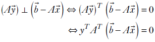
For the previous equation to be true for all vectors ![]() , we must have AT(
, we must have AT(![]() −A
−A![]() ) = 0.
) = 0.
Thus, we have
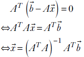
which is exactly the Moore-Penrose pseudo-inverse.
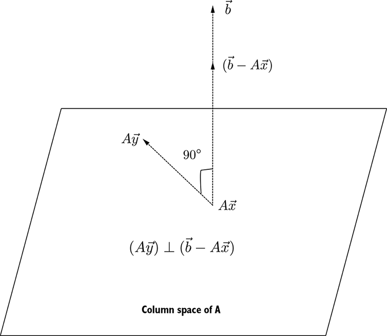
Figure 2.12 Solving a linear system A![]() =
= ![]() is equivalent to finding the point on the column space of A that is closest to
is equivalent to finding the point on the column space of A that is closest to ![]() . This means we have to drop a perpendicular from
. This means we have to drop a perpendicular from ![]() to column space of A. If A
to column space of A. If A![]() represents the point where that perpendicular meets the column space (aka projection), the difference vector
represents the point where that perpendicular meets the column space (aka projection), the difference vector ![]() − A
− A![]() corresponds to the line joining
corresponds to the line joining ![]() and its projection A
and its projection A![]() . This line will be perpendicular to all vectors in the column space of A. Equivalently, it is perpendicular to A
. This line will be perpendicular to all vectors in the column space of A. Equivalently, it is perpendicular to A![]() for any arbitrary
for any arbitrary ![]() .
.
For a machine learning-centric example, consider the overdetermined system corresponding to the cat brain earlier in the chapter. There are 15 training examples, each with input and desired outputs specified.
Our goal is to determine three unknowns w0, w1, and b such that for each training input ![]() , the model output
, the model output
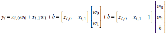
Equation 2.20
matches the desired output (aka ground truth) ȳi as closely as possible.
NOTE We employed a neat trick here: we added a 1 to the right of the input, which allows us to depict the entire system (including the bias) in a single compact matrix-vector multiplication. We call this augmentation—we augment the input row vector with an extra 1 on the right.
Collating all the training examples together, we get
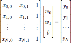
Equation 2.21
which can be expressed compactly as
X![]() =
= ![]()
where X is the augmented input matrix with a rightmost column of all 1s. The goal is to minimize ||![]() –
– ![]() ||. To this end, we formulate the over-determined linear system
||. To this end, we formulate the over-determined linear system
X![]() =
= ![]()
Note that this is not a classic system of equations—it has more equations than unknowns. We cannot solve this via matrix inversion. We can, however, use the pseudo-inverse mechanism to solve it. The resulting solution yields the “best fit” or “best effort” solution, which minimizes the total error over all the training examples.
The exact numerical system (repeated here for ease of reference) is
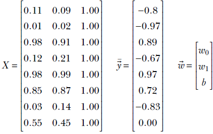
Equation 2.22
We solve for ![]() using the pseudo-inverse formula
using the pseudo-inverse formula ![]() = (XTX)–1XT
= (XTX)–1XT![]()
2.12.6 PyTorch code to solve overdetermined systems
NOTE Fully functional code for this section, executable via Jupyter Notebook, can be found at http://mng.bz/PPJ2.
Listing 2.12 Solving an overdetermined system using the pseudo-inverse
def pseudo_inverse(A):
    return torch.matmul(torch.linalg.inv(torch.matmul(A.T, A)), A.T)

①
X = torch.column_stack((X, torch.ones(15))) ②

③
w = torch.matmul(pseudo_inverse(X), y)      ④

print("The solution is {}".format(w))       ⑤
① X is the augmented data matrix from equation 2.22
② The Pytorch column stack operator
adds a column to a matrix. Here, the added column is all 1s
③ It is easy to verify that the solution to equation 2.22 is roughly w0 = 1, w1 = 1, b = −1. But the equations are not consistent: no one solution perfectly fits all of them. The pseudo-inverse finds the “best fit” solution: it minimizes total error for all the equations.
④ Expect the solution to be close to [1, 1, −1]
⑤ The solution is [1.08, 0.90, −0.96]
2.13 Eigenvalues and eigenvectors: Swiss Army knives of machine learning
Machine learning and data science are all about finding patterns in large volumes of high-dimensional data. The inputs are feature vectors introduced in section 2.1) in high-dimensional spaces. Each feature vector can be viewed as a point in the feature space descriptor for an input instance. Sometimes we transform these feature vectors—map the feature points to a friendlier space—to simplify the data by reducing dimensionality. This is done by eliminating axes along which there is scant variation in the data. Eigenvalues and eigenvectors are invaluable tools in the arsenal of a machine learning engineer or a data scientist for this purpose. In chapter 4, we will study how to use these tools to simplify and find broad patterns in a large volume of multidimensional data.
Let’s take an informal look at eigenvectors first. They are properties of square matrices. As seen earlier, matrices can be viewed as linear transforms which map vectors (points) in one space to different vectors (points) in the same or a different space. But a typical linear transform leaves a few points in the space (almost) unaffected. These points are called eigenvectors. They are important physical aspects of the transform. Let’s look at a simple example. Suppose we are rotating points in 3D space about the Z-axis (see figure 2.13). The points on the Z-axis will stay where they were despite the rotation. In general, points on the axis of rotation (Z in this case) do not go anywhere after rotation. The axis of rotation is an eigenvector of the rotation transformation.
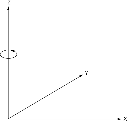
Figure 2.13 During rotation, points on the axis of rotation do not change position.
Extending this idea, when transforming vectors ![]() with a matrix A, are there vectors that do not change, at least in direction? Turns out the answer is yes. These are the so-called eigenvectors—they do not change direction when undergoing linear transformation by a matrix A. To be precise, if
with a matrix A, are there vectors that do not change, at least in direction? Turns out the answer is yes. These are the so-called eigenvectors—they do not change direction when undergoing linear transformation by a matrix A. To be precise, if ![]() is an eigenvector of the square matrix A, 5 then
is an eigenvector of the square matrix A, 5 then
A![]() = λ
= λ![]()
Thus the linear transformation (that is, multiplication by matrix A) has changed the length but not the direction of ![]() because λ
because λ![]() is parallel to
is parallel to ![]() .
.
How do we obtain λ and ![]() ? Well,
? Well,
A![]() = λ
= λ ![]()
⇔ A![]() - λ
- λ![]() =
= ![]()
⇔ (A - λ I)![]() =
= ![]()
where I denotes the identity matrix.
Of course, we are only interested in nontrivial solutions, where ![]() ≠
≠ ![]() . In that case, A – λI cannot be invertible, because if it were, we could obtain the contradictory solution
. In that case, A – λI cannot be invertible, because if it were, we could obtain the contradictory solution ![]() = (A – λ I)–1
= (A – λ I)–1 ![]() =
= ![]() . Thus, (A − λI) is non-invertible, implying the determinant
. Thus, (A − λI) is non-invertible, implying the determinant
det(A − λI) = 0
For an n × n matrix A, this yields an nth-degree polynomial equation with n solutions for the unknown λ. Thus, an n × n matrix has n eigenvalues, not necessarily all distinct.
Let’s compute eigenvalues and eigenvectors of a 3 × 3 matrix, just for kicks. The matrix we use is carefully chosen, as will be evident soon. But for now, think of it as an arbitrary matrix:
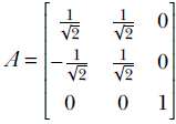
Equation 2.23
We will compute the eigenvalues and eigenvectors of A:
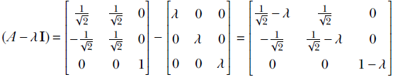
Thus,
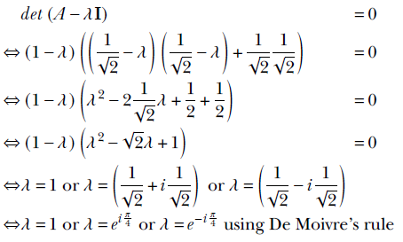
Here, i = √–1. If necessary, you are encouraged to refresh your memory of imaginary and complex numbers from high school algebra.
Thus, we have found (as expected) three eigenvalues: 1, ei π/4, and e–i π/4. Each of them will yield one eigenvector. Let’s compute the eigenvector corresponding to the eigenvalue of 1 by way of example:
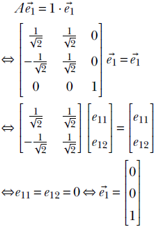
Thus, ![]() is an eigenvector for the eigenvalue 1 for matrix A. So is
is an eigenvector for the eigenvalue 1 for matrix A. So is ![]() for any real k. In fact, if λ,
for any real k. In fact, if λ, ![]() is an eigenvalue, eigenvector pair for matrix A, then
is an eigenvalue, eigenvector pair for matrix A, then
A![]() = λ
= λ![]() ⇔ A(k
⇔ A(k![]() ) = λ(k
) = λ(k![]() )
)
That is, λ, (k![]() ) is also an eigenvalue, eigenvector pair of A. In other words, we can only determine the eigenvector up to a fixed scale factor. We take the eigenvector to be of unit length (
) is also an eigenvalue, eigenvector pair of A. In other words, we can only determine the eigenvector up to a fixed scale factor. We take the eigenvector to be of unit length (![]() T
T![]() = 1) without loss of generality.
= 1) without loss of generality.
The eigenvector for our example matrix turns out to be the Z-axis. This is not an accident. Our matrix A was, in fact, a rotation about the Z-axis. A rotation matrix will always have 1 as an eigenvalue. The corresponding eigenvector will be the axis of rotation. In 3D, the other two eigenvalues will be complex numbers yielding the angle of rotation. This is detailed in section 2.14.
2.13.1 Eigenvectors and linear independence
Two eigenvectors of a matrix corresponding to unequal eigenvalues are linearly independent. Let’s prove this to get some insights. Let λ1, ![]() 1 and λ2,
1 and λ2, ![]() 2 be eigenvalue, eigenvector pairs for a matrix A with λ1 ≠ λ2. Then
2 be eigenvalue, eigenvector pairs for a matrix A with λ1 ≠ λ2. Then
A![]() 1 = λ1
1 = λ1![]() 1
1
A![]() 2 = λ2
2 = λ2![]() 2
2
If possible, let there be two constants α1 and α2 such that
α1![]() 1 + α2
1 + α2![]() 2 = 0
2 = 0
Equation 2.24
In other words, suppose the two eigenvectors are linearly dependent. We will show that this assumption leads to an impossibility.
Multiplying equation 2.24 by A, we get
α1A![]() 1 + α2A
1 + α2A![]() 2 = 0
2 = 0
⇔ α1λ1![]() 1 + α2λ2
1 + α2λ2![]() 2 = 0
2 = 0
Also, we can multiply equation 2.24 by λ2. Thus we get
α1λ1![]() 1 + α2λ2
1 + α2λ2![]() 2 = 0
2 = 0
α1λ2![]() 1 + α2λ2
1 + α2λ2![]() 2 = 0
2 = 0
Subtracting, we get
α1(λ1-λ2)![]() 1 = 0
1 = 0
By assumption, α1 ≠ 0, λ1 ≠ λ2 and ![]() 1 is not all zeros. Thus it is impossible for their product to be zero. Our original assumption (the two eigenvectors are linearly dependent) must have been wrong.
1 is not all zeros. Thus it is impossible for their product to be zero. Our original assumption (the two eigenvectors are linearly dependent) must have been wrong.
2.13.2 Symmetric matrices and orthogonal eigenvectors
Two eigenvectors of a symmetric matrix that correspond to different eigenvalues are mutually orthogonal. Let’s prove this to get additional insight. A matrix A is symmetric if AT = A. If λ1, ![]() 1 and λ2,
1 and λ2, ![]() 2 are eigenvalue, eigenvector pairs for a symmetric matrix A, then
2 are eigenvalue, eigenvector pairs for a symmetric matrix A, then
A![]() 1 = λ1
1 = λ1![]() 1
1
Equation 2.25
A![]() 2 = λ2
2 = λ2![]() 2
2
Equation 2.26
Transposing equation 2.25,
![]() 1T AT = λ1
1T AT = λ1![]() 1T
1T
Right-multiplying by ![]() 2, we get
2, we get
![]() 1T AT
1T AT![]() 2 = λ1
2 = λ1![]() 1T
1T ![]() 2
2
⇔ ![]() 1T A
1T A![]() 2 = λ1
2 = λ1![]() 1T
1T ![]() 2
2
where the last equation follows from the matrix symmetry. Also, left-multiplying equation 2.26 by ![]() 1T, we get
1T, we get
![]() 1T A
1T A![]() 2 = λ2
2 = λ2![]() 1T
1T ![]() 2
2
Thus
![]() 1T A
1T A![]() 2 = λ1
2 = λ1![]() 1T
1T ![]() 2
2
![]() 1T A
1T A![]() 2 = λ2
2 = λ2![]() 1T
1T ![]() 2
2
Subtracting the equations, we get
0 = (λ1 - λ2) ![]() 1T
1T ![]() 2
2
Since λ1 ≠ λ2, we must have ![]() 1T
1T ![]() 2 = 0, which means the two eigenvectors are orthogonal. Thus, if A is an n × n symmetric matrix with eigenvectors
2 = 0, which means the two eigenvectors are orthogonal. Thus, if A is an n × n symmetric matrix with eigenvectors ![]() 1,
1, ![]() 2, …
2, … ![]() n, then
n, then ![]() iT
iT![]() j = 0 for all i, j satisfying λi ≠ λj.
j = 0 for all i, j satisfying λi ≠ λj.
2.13.3 PyTorch code to compute eigenvectors and eigenvalues
NOTE Fully functional code for this section, executable via Jupyter Notebook, can be found at http://mng.bz/1rEZ.
Listing 2.13 Eigenvalues and vectors
from torch import linalg as LA

A = torch.tensor([[0.707, 0.707, 0],
       [-0.707, 0.707, 0], [0, 0, 1]])    ①

l, e = LA.eig(A)                          ②

print("Eigen values are {}".format(l))
print("Eigen vectors are {}".format(e.T)) ③
① 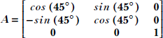 Rotates points in 3D space around the Z-axis.
The axis of rotation is the Z-axis: [0 0 1]T
② Function eig() in the torch linalg package computes eigenvalues and vectors.
③ Eigenvalues or vectors can contain complex numbers involving j = √-1
2.14 Orthogonal (rotation) matrices and their eigenvalues and eigenvectors
Of all the transforms, rotation transforms have a special intuitive appeal because of their highly observable behavior in the mechanical world. Furthermore, they play a significant role in developing and analyzing several machine learning tools. In this section, we overview rotation (aka orthogonal) matrices. (Fully functional code for the Jupyter notebook for this section can be found at http://mng.bz/2eNN.)
2.14.1 Rotation matrices
Figure 2.14 shows a point (x, y) rotated about the origin by an angle θ. The original point’s position vector made an angle α with the X-axis. Post-rotation, the point’s new coordinates are (x′, y′). Note that by definition, rotation does not change the distance from the center of rotation; that is what the circle indicates.
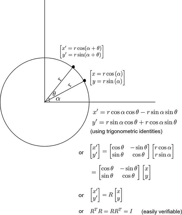
Figure 2.14 Rotation in a plane about the origin. By definition, rotation does not change the distance from the center of rotation (indicated by the circle).
Some well-known rotation matrices are as follows:
-
Planar rotation by angle θ about the origin (see figure 2.14):
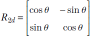
Equation 2.27
-
Rotation by angle θ in 3D space about the Z-axis:
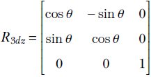
Equation 2.28
Note that the z coordinate remains unaffected by this rotation:
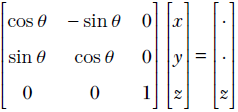
This rotation matrix has an eigenvalue of 1, and the corresponding eigenvector is the Z-axis—you should verify this. This implies that a point on the Z-axis maps to itself when transformed (rotated) by the previous matrix, which is in keeping with the property that the z coordinate remains unchanged by this rotation.
-
Rotation by angle θ in 3D space about the X-axis:
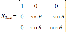
Equation 2.29
Note that the X coordinate remains unaffected by this rotation and the X-axis is an eigenvector of this matrix:
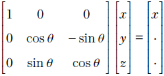
-
Rotation by angle θ in 3D space about the Y-axis:
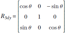
Equation 2.30
Note that the Y coordinate remains unaffected by this rotation and the Y-axis is an eigenvector of this matrix:
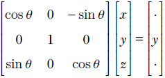
Listing 2.14 Rotation matrices
def rotation_matrix_2d(theta):                                            ①
     return torch.tensor([[cos(radians(theta)), -sin(radians(theta))],
                      [sin(radians(theta)), cos(radians(theta))]])

def rotation_matrix_3d(theta, axis):                                      ②
     if axis == 0:                                                        ③
       return torch.tensor([[1, 0, 0],
                        [0, cos(radians(theta)),-sin(radians(theta))],
                        [0, sin(radians(theta)),cos(radians(theta))]])
     elif axis == 1:                                                      ④
       return torch.tensor([[cos(radians(theta)),0,-sin(radians(theta))],
                        [0, 1, 0],
                        [sin(radians(theta)),0,cos(radians(theta))]])
     elif axis == 2:                                                      ⑤
       return torch.tensor([[cos(radians(theta)),-sin(radians(theta)),0],
                        [sin(radians(theta)),cos(radians(theta)),0],
                        [0, 0, 1]])
① Returns the matrix that performs in-plane 2D rotation by angle theta about the origin. Thus, multiplication with this matrix moves a point to a new location. The angle between the position vectors of the original and new points is theta (figure 2.14).
② Returns the matrix that rotates a point in 3D space about the chosen axis by angle theta degrees. The axis of rotation can be 0, 1, or 2, corresponding to the X-, Y-, or Z-axis, respectively.
③ R3dx from equation 2.29
④ R3dy from equation 2.30
⑤ R3dz from equation 2.28
Listing 2.15 Applying rotation matrices
u = torch.tensor.array([1, 1, 1], dtype=torch.float)  ①

R3dz = rotation_matrix_3d(45, 2)                      ②
v = torch.matmul(R3dz, u_row)                         ③

R3dx = rotation_matrix_3d(45, 0)                      ④
w = torch.matmul(R3dx, u_row)                         ⑤
① Creates vector ![]() (see figure 2.15)
(see figure 2.15)
② R3dz from equation 2.28, 45° about Z-axis
③ ![]() (see figure 2.15) is
(see figure 2.15) is ![]() rotated by R3dz.
rotated by R3dz.
④ R3dx from equation 2.28, 45° about X-axis
⑤ ![]() (see figure 2.15) is
(see figure 2.15) is ![]() rotated by R3dx.
rotated by R3dx.
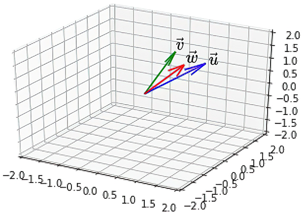
Figure 2.15 Rotation visualized. Here the original vector u is first rotated by 45 degrees around the Z-axis to get vector v, which is subsequently rotated again by 45 degrees around the X-axis to get vector w.
2.14.2 Orthogonality of rotation matrices
A matrix R is orthogonal if and only if it its transpose is also its inverse: that is, RTR = RRT = I. All rotations matrices are orthogonal matrices. All orthogonal matrices represent some rotation. For instance:

You are encouraged to verify, likewise, that all the rotation matrices shown here are orthogonal.
Orthogonality and length-preservation
Orthogonality implies that rotation is length-preserving. Given any vector ![]() and rotation matrix R, let
and rotation matrix R, let ![]() = R
= R![]() be the rotated vector. The lengths (magnitudes) of the two vectors
be the rotated vector. The lengths (magnitudes) of the two vectors ![]() ,
, ![]() are equal since it is easy to see that
are equal since it is easy to see that
||![]() || =
|| = ![]() T
T![]() = (R
= (R![]() )T(R
)T(R![]() ) =
) = ![]() TRTR
TRTR![]() =
= ![]() TI
TI![]() =
= ![]() T
T![]() = ||
= ||![]() ||
||
From elementary matrix theory, we know that
(AB)T = BTAT
Negating the angle of rotation
Negating the angle of rotation is equivalent to inverting the rotation matrix, which is equivalent to transposing the rotation matrix. For instance, consider in-plane rotation. Say a point ![]() is rotated about the origin to vector
is rotated about the origin to vector ![]() via matrix R. Thus
via matrix R. Thus
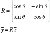
Now we can go back from ![]() to
to ![]() by rotating by −θ. The corresponding rotation matrix is
by rotating by −θ. The corresponding rotation matrix is
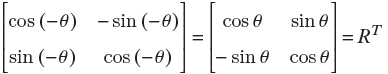
In other words, RT inverts the rotation: that is, rotates by the negative angle.
2.14.3 PyTorch code for orthogonality of rotation matrices
Let’s verify the orthogonality of the rotation matrix by creating one in PyTorch, imparting a transpose to it, and verifying that the product of the original matrix and the transpose is the identity matrix.
Listing 2.16 Orthogonality of rotation matrices
R_30 = rotation_matrix_2d(30)                      ①

assert torch.allclose(
    torch.linalg.inv(R_30),
    R_30.T

    )                                              ②

assert torch.allclose(
    torch.matmul(R_30, R_30.T),
    torch.eye(2)                                   ③
    )

u = torch.tensor([[4],[0]], dtype=torch.float)

v = torch.matmul(R_30, u)                          ④

assert torch.linalg.norm(u) ==torch.linalg.norm(v)  ⑤

R_neg30 = rotation_matrix_2d(-30)
w = torch.matmul(R_neg30, v)                       ⑥
assert torch.all(w == u)

assert torch.allclose(R_30, R_neg30.T)
assert torch.allclose(
    torch.matmul(R_30, R_neg30),
    torch.eye(2))                                  ⑦
① Creates a rotation matrix, R30
② The inverse of a rotation matrix is the same as its transpose.
③ Multiplying a rotation matrix and its inverse yields the identity matrix.
④ A vector ![]() rotated by matrix R30 to yield vector
rotated by matrix R30 to yield vector ![]() , R30
, R30![]() =
= ![]() .
.
⑤ The norm of a vector is the same as its length. Rotation preserves the length of a vector ||R![]() || = ||
|| = ||![]() ||.
||.
⑥ Rotation by an angle followed by rotation by the negative of that angle takes the vector back to its original position. Rotation by a negative angle is equivalent to inverse rotation.
⑦ A matrix that rotates by an angle is the inverse of the matrix that rotates by the negative of the same angle.
2.14.4 Eigenvalues and eigenvectors of a rotation matrix:Finding the axis of rotation
Let λ, ![]() be an eigenvalue, eigenvector pair of a rotation matrix R. Then R
be an eigenvalue, eigenvector pair of a rotation matrix R. Then R![]() = λ
= λ![]()
Transposing both sides,
![]() TRT = λ
TRT = λ![]() T
T
Multiplying the left and right sides, respectively, with the equivalent entities R![]() and λ
and λ![]() , we get
, we get
![]() TRT(R
TRT(R![]() ) = λ
) = λ![]() T(λ
T(λ![]() ) ⇔
) ⇔ ![]() T(RTR)
T(RTR)![]() = λ2
= λ2![]() T
T![]() ⇔
⇔ ![]() T(I)
T(I)![]() = λ2
= λ2![]() T
T![]()
⇔ ![]() T
T![]() = λ2
= λ2![]() T
T![]() ⇔ λ2 = 1 ⇔ λ = 1
⇔ λ2 = 1 ⇔ λ = 1
(The negative solution λ = −1 corresponds to reflection.) Thus, all rotation matrices have 1 as one of their eigenvalues. The corresponding eigenvector ![]() satisfies R
satisfies R![]() =
= ![]() . This is the axis of rotation: the set of points that stay where they were post-rotation.
. This is the axis of rotation: the set of points that stay where they were post-rotation.
2.14.5 PyTorch code for eigenvalues and vectors of rotation matrices
The following listing shows the code for the axis of rotation.
Listing 2.17 Axis of rotation
R = torch.tensor([[0.7071, 0.7071, 0],
             [-0.7071, 0.7071, 0],                      ①
             [0, 0, 1]])

l, e = LA.eig(R)                                        ②

③
axis_of_rotation = e[:, torch.where(l == 1.0)]          ④

axis_of_rotation = torch.squeeze(axis_of_rotation)

assert torch.allclose(
    axis_of_rotation.real,
    torch.tensor([0, 0, 1], dtype=torch.float)          ⑤
)

p = torch.randint(0, 10, (1,)) * axis_of_rotation
assert torch.allclose(torch.matmul(R, p.real), p.real)  ⑥
① 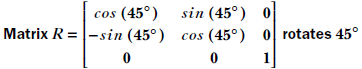
about the Z-axis. All rotation matrices will havean eigenvalue 1. The corresponding eigenvector
is the axis of rotation (here, the Z-axis).
② The PyTorch function eig() computes eigenvalues and eigenvectors.
③ The PyTorch function where() returns the indices at which the specified condition is true.
④ Obtains the eigenvector for eigenvalue 1
⑤ The axis of rotation is the Z-axis.
⑥ Takes a random point
on this axis and applies the rotation to this point; its position does not change.
2.15 Matrix diagonalization
In section 2.12, we studied linear systems and their importance in machine learning. We also remarked that the standard mathematical process of solving linear systems via matrix inversion is not very desirable from a machine learning point of view. In this section, we will see one method of solving linear systems without matrix inversion. In addition, this section will help us develop the insights necessary to understand quadratic forms and, eventually, principal component analysis (PCA), one of the most important tools in data science.
Consider an n × n matrix A with n linearly independent eigenvectors. Let S be a matrix with these eigenvectors as its columns. That is,
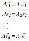
and
![]()
Then
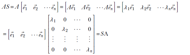
where
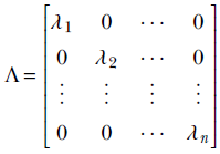
is a diagonal matrix with the eigenvalues of A on the diagonal and 0 everywhere else.
Thus, we have
AS = SΛ
which leads to
A = SΛS−1
and
Λ = S−1AS
If A is symmetric, then its eigenvectors are orthogonal. Then STS = SST = I ⇔ S−1 = ST, and we get the diagonalization of A: A = SΛST Note that diagonalization is not unique: a given matrix may be diagonalized in multiple ways.
2.15.1 PyTorch code for matrix diagonalization
Now we will study the PyTorch implementation of the math we learned in section 2.15. As usual, we will only show the directly relevant bit of code here.
NOTE Fully functional code for this section, executable via Jupyter Notebook, can be found at http://mng.bz/RXJn.
Listing 2.18 Diagonalization of a matrix
def diagonalize(matrix):                              ①

    try:
        l, e = torch.linalg.eig(matrix)               ②


        sigma = torch.diag(l)                         ③

        return e, torch.diag(l), torch.linalg.inv(e)  ④
    except np.linalg.LinAlgError:
        print("Cannot diagonalize matrix!")

A = torch.tensor([[0.7071, 0.7071, 0],
              [-0.7071, 0.7071, 0],                   ⑤
              [0, 0, 1]])

S, sigma, S_inv = diagonalize(A)

A1 = torch.matmul(S, torch.matmul(sigma, S_inv))      ⑥

assert torch.allclose(A, A1.real)                     ⑦
① Diagonalization is factorizing a matrix A = SΣS−1. S is a matrix with eigenvectors of A as columns. Σ is a diagonal matrix with eigenvalues of A in the diagonal.
② The PyTorch function eig() returns eigenvalues and vectors.
③ The PyTorch function diag() creates a diagonal matrix of given values.
④ Returns the three factors
⑤ Creates a matrix A
⑥ Reconstructs A from its factors
⑦ Verifies that the reconstructed matrix is the same as the original
2.15.2 Solving linear systems without inversion via diagonalization
Diagonalization has many practical applications. Let’s study one now. In general, matrix inversion (that is, computing A−1) is a very complex process that is numerically unstable. Hence, solving A![]() =
= ![]() via
via ![]() = A−1
= A−1![]() is to be avoided when possible. In the case of a square symmetric matrix with n distinct eigenvalues, diagonalization can come to the rescue. We can solve this in multiple steps. We first diagonalize A:
is to be avoided when possible. In the case of a square symmetric matrix with n distinct eigenvalues, diagonalization can come to the rescue. We can solve this in multiple steps. We first diagonalize A:
A = SΛST
Then
A![]() =
= ![]()
can be written as:
SΛST![]() =
= ![]()
where S is the matrix with eigenvectors of A as its columns:
S = [![]() 1
1 ![]() 2 …
2 … ![]() n]
n]
(Since A is symmetric, these eigenvectors are orthogonal. Hence STS = SST = I.) The solution can be obtained in a series of very simple steps:
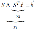
First solve
S![]() 1 =
1 = ![]()
as
![]() 1 = ST
1 = ST ![]()
Notice that both the transpose and matrix-vector multiplications are simple and numerically stable operations, unlike matrix inversion. Then we get
Λ(ST![]() ) =
) = ![]() 1
1
Now solve
Λ![]() 2 =
2 = ![]() 1
1
as
![]() 2 = Λ–1
2 = Λ–1![]() 1
1
Note that since Λ is a diagonal matrix, inverting it is trivial:
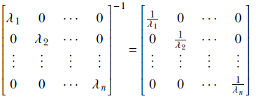
Equation 2.31
As a final step, solve
ST![]() =
= ![]() 2
2
as
![]() = S
= S![]() 2
2
Thus we have obtained ![]() without a single complex or unstable step.
without a single complex or unstable step.
2.15.3 PyTorch code for solving linear systems via diagonalization
Let’s try solving the following set of equations:
x + y + z = 8
2x + 2y + 3z = 15
x + 3y + 3z = 16
This can be written using matrices and vectors as
A![]() =
= ![]()
where
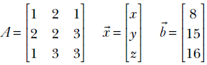
Note that A is a symmetric matrix. It has orthogonal eigenvectors. The matrix with eigenvectors of A in columns is orthogonal. Its transpose and inverse are the same.
Listing 2.19 Solving linear systems using diagonalization
A = torch.tensor([[1, 2, 1], [2, 2, 3], [1, 3, 3]],
                        dtype=torch.float)         ①
assert torch.all(A == A.T)                         ②
b = torch.tensor([8, 15, 16], dtype=torch.cfloat)  ③

x_0 = torch.matmul(torch.linalg.inv(A),
                                b.real)            ④

w, S = torch.linalg.eig(A)                         ⑤

 1 = torch.matmul(S.T, b)                          ⑥

 2 = torch.matmul(torch.diag(1/ w), y1)            ⑦

x_1 = torch.matmul(S, y2)                          ⑧

assert torch.allclose(x_0, x_1.real)               ⑨
① Creates a symmetric matrix A
② Asserts that A may be symmetric
③ Creates a vector ![]()
④ Solves A![]() =
= ![]() using matrix inversion,
using matrix inversion, ![]() = A−1
= A−1![]() .
.
Note: matrix inversion is numerically unstable.
⑤ Solves A![]() =
= ![]() via diagonalization. A = SΣST.
via diagonalization. A = SΣST.
 .
.
⑥ 1. Solve: S![]() 1 =
1 = ![]() as
as ![]() 1 = ST
1 = ST ![]() (no matrix inversion)
(no matrix inversion)
⑦ 2. Solve: Λ ![]() 2 =
2 = ![]() 1 as
1 as ![]() 2 = Λ-1
2 = Λ-1![]() 1 (inverting a diagonal matrix is easy; see equation 2.31.)
1 (inverting a diagonal matrix is easy; see equation 2.31.)
⑧ 3. Solve: ST![]() =
= ![]() 2 as
2 as ![]() = S
= S![]() 2 (no matrix inversion)
2 (no matrix inversion)
⑨ Verifies that the two solutions are the same
⑨ Verifies that the two solutions are the same
2.15.4 Matrix powers using diagonalization
If matrix A can be diagonalized, then
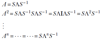
For a diagonal matrix
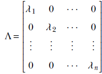
the nth power is simply
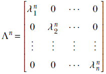
If we need to compute various powers of an m × m matrix A at different times, we should precompute the matrix S and compute any power with only O(m) operations—compared to the (nm3) operations necessary for naive computations.
2.16 Spectral decomposition of a symmetric matrix
We have seen in section 2.15 that a square symmetric matrix with distinct eigenvalues can be decomposed as
A = SΛST
where
A = [![]() 1
1 ![]() 2 …
2 … ![]() n]
n]
Thus,
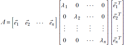
This equation can be rewritten as
A = λ1![]() 1
1![]() 1T + λ2
1T + λ2![]() 2
2![]() 2T + … + λn
2T + … + λn![]() n
n![]() nT
nT
Equation 2.32
Thus a square symmetric matrix can be written in terms of its eigenvalues and eigenvectors. This is the spectral resolution theorem.
2.16.1 PyTorch code for the spectral decomposition of a matrix
The following listing shows the relevant code for this section.
Listing 2.20 Spectral decomposition of a matrix
def spectral_decomposition(A):
  assert len(A.shape) == 2                                    ①

     and A.shape[0] == A.shape[1]                             ②

     and torch.all(A == A.T)                                  ③

  l, e = torch.linalg.eig(A)                                  ④

  assert len(torch.unique(l.real)) == A.shape[0],
         ``Eigen values are not distinct!"

  C = torch.zeros((A.shape[0],
                          A.shape[0],                         ⑤
                          A.shape[0]))

  for i, lambda_i in enumerate(l):
      e_i = e[:, i]
      e_i = e_i.reshape((3, 1))
      C[i, :, :] = (lambda_i * torch.matmul(e_i, e_i.T)).real ⑥
  return C

A = torch.tensor([[1, 2, 1], [2, 2, 3], [1, 3, 3]]).float()
C = spectral_decomposition(A)

A1 = C.sum(axis=0)                                            ⑦

assert torch.allclose(A, A1)                                  ⑧
① Asserts that A is a 2D tensor (i.e., matrix)
② A is square: i.e., A.shape[0] (num rows) ≜ A.shape[1] (num columns)
③ Asserts that A is symmetric: i.e., A = = AT
④ The PyTorch function eig() returns eigenvectors and values.
⑤ Defines a 3D tensor C of shape n × n × n to hold the n components from equation 2.32. Each term λi![]() i
i![]() T is an n × n matrix. There are n such terms, all compactly held in tensor C.
T is an n × n matrix. There are n such terms, all compactly held in tensor C.
⑥ Computes C[i] = λi![]() i
i![]() T
T
⑦ Reconstructs A by adding its components stored in C
⑧ Verifies that the matrix reconstructed from spectral components matches the original
2.17 An application relevant to machine learning: Finding the axes of a hyperellipse
The notion of an ellipse in high-dimensional space (aka hyperellipse) keeps coming back in various forms in machine learning. Here we will make a preliminary review of them. We will revisit these concepts later.
Recall the equation of an ellipse from high school math:

This is a rather simple ellipse: it is two-dimensional and centered at the origin, and its major and minor axes are aligned with the coordinate axes. Denoting ![]() as the position vector, the same equation can be written as
as the position vector, the same equation can be written as
![]() TΛ
TΛ![]() = 1
= 1
where 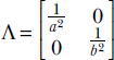 is a diagonal matrix. Written in this form, the equation can be extended beyond 2D to an n-dimensional axis-aligned ellipse centered at the origin. Now let’s apply a rotation R to the axis. Then every vector
 ![]() transforms to R
transforms to R![]() . The equation of the ellipse in the new (rotated) coordinate system is
. The equation of the ellipse in the new (rotated) coordinate system is
(R![]() T Λ (R
T Λ (R![]() ) = 1
) = 1
⇔ ![]() T (RT ΛR)
T (RT ΛR) ![]() = 1
= 1
where
A = (RTΛR).
The generalized equation of the ellipse is
![]() TA
TA![]() = 1
= 1
Note the following:
-
The ellipse is no longer axis aligned.
-
The matrix A is no longer diagonal.
-
A is symmetric. We can easily verify that AT = (RTΛR)T = RTΛTR = RTΛR (remember, the transpose of a diagonal matrix is itself).
If, in addition, we want to get rid of the “centered at the origin” assumption, we get
(![]() −μ)TA(
−μ)TA(![]() −μ) = 1
−μ) = 1
Equation 2.33
Now let’s flip the problem around. Suppose we have a generic n-dimensional ellipse. How do we compute its axes’ directions?
Clearly, if we can rotate the coordinate system so that the matrix in the middle is diagonal, we are done. Diagonalization (see section 2.15) is the answer. Specifically, we find the matrix S with eigenvectors of A in its columns. This is a rotation matrix (being orthogonal, since A is symmetric). We transform rotate) the coordinate system by applying this matrix. In this new coordinate system, the ellipse is axis aligned. Stated another way, the new coordinate axes—these are the eigenvectors of A—yield the axes of the ellipse.
2.17.1 PyTorch code for hyperellipses
Let’s try finding the axes of the hyperellipse described by the equation 5x2 + 6xy + 5y2 = 20. Note that the actual ellipse we use as an example is 2D (to facilitate visualization), but the code we develop will be general and extensible to multiple dimensions.
The ellipse equation can be written using matrices and vectors as ![]() TA
TA![]() = 1, where
= 1, where
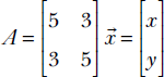
To find the axes of the hyperellipse, we need to transform the coordinate system so that the matrix in the middle becomes diagonal. Here is how this can be done: if we diagonalize A into SΣS−1, then the ellipse equation becomes ![]() TSΣS−1
TSΣS−1![]() = 1, where Σ is a diagonal matrix. Since A is symmetric, its eigenvectors are orthogonal. Hence, the matrix containing these eigenvectors as columns is orthogonal: i.e., S−1 = ST. In other words, S is a rotation matrix. So the ellipse equation becomes
= 1, where Σ is a diagonal matrix. Since A is symmetric, its eigenvectors are orthogonal. Hence, the matrix containing these eigenvectors as columns is orthogonal: i.e., S−1 = ST. In other words, S is a rotation matrix. So the ellipse equation becomes ![]() TSΣST
TSΣST![]() = 1 or (
= 1 or (![]() TS)Σ(ST
TS)Σ(ST![]() ) = 1 or
) = 1 or ![]() TΣ
TΣ![]() = 1 where
= 1 where ![]() = ST
= ST![]() . This is of the desired form since Σ is a diagonal matrix. Remember, S is a rotation matrix. Thus, rotating the coordinate system by S aligns the coordinate axes with the ellipse axes.
. This is of the desired form since Σ is a diagonal matrix. Remember, S is a rotation matrix. Thus, rotating the coordinate system by S aligns the coordinate axes with the ellipse axes.
Listing 2.21 Axes of a hyperellipse
ellipse_eq = sy.Eq(5*x**2 + 5*y**2 +
                      6*x*y, 20)                   ①

A = torch.tensor([[5, 3], [3, 5]]).float()

l, S = torch.linalg.eig(A)

x_axis_vec = torch.zeros((A.shape[0]))             ②

first_eigen_vec = S[:, 0]                          ③

dot_prod = torch.dot(x_axis_vec, first_eigen_vec)  ④

theta = math.acos(dot_prod)
theta = math.degrees(theta)                        ⑤
① Equation of the ellipse: 5x2 + 6xy + 5y2 = 20 or ![]() TA
TA![]() = 20, where
= 20, where ![]()
② X-axis vector
③ Major axis of the ellipse
④ The dot product between two vectors is the cosine of the angle between them.
⑤ The angle between the ellipse’s major axis and the X-axis: 45° (see figure 2.16)
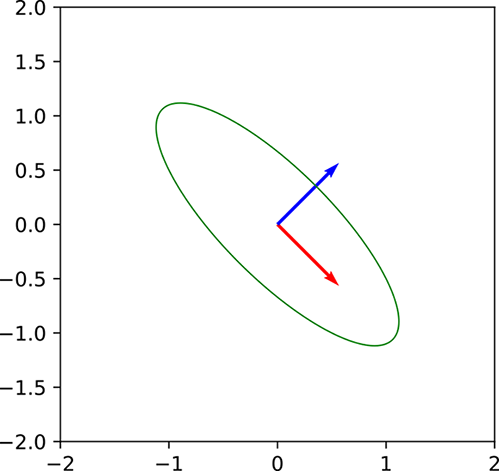
Figure 2.16 Note that the ellipse’s major axis forms an angle of 45 degrees with the X-axis. Rotating the coordinate system by this angle will align the ellipse axes with the coordinate axes. Subsequently, the first principal vector will also lie along this direction.
Summary
-
In machine learning, a vector is a one-dimensional array of numbers and a matrix is a two-dimensional array of numbers. Inputs and outputs of machine learning models are typically represented as vectors or matrices. In multilayered models, inputs and outputs of each individual layer are also represented as vectors or matrices. Images are two-dimensional arrays of numbers corresponding to pixel color values. As such, they are represented as matrices.
-
An n-dimensional vector can be viewed as point in ℝn space. All models can be viewed as functions that map points from input to output space. The model is designed so that it is easier to solve the problem of interest in the output space.
-
A dot product between a pair of vectors
= [x1 x2 … xn] and  = [y1 y2 … yn] is the scalar quantity ⋅ = x1y1 + x2y2 + ⋯ + xnyn. It is a measure of how similar the vectors are. Dot products are widely used in machine learning. For instance, in supervised machine learning, we train the model so that its output is as similar as possible to the known output for a sample set of input points known as training data. Here, some variant of the dot product is often used to measure the similarity of the model output and the known output. Two vectors are orthogonal if their dot product is zero. This means the vectors have no similarity and are independent of each other.
A vector’s dot product with itself is the square of the magnitude or length of the vector ⋅ = ||||2 = x1x1 + x2x2 + ⋯ + xnxn. -
Given a set of vectors
1, 2, ⋯, n, the weighted sum a11 + a22 + ⋯ + ann where a1, a2, ⋯, an are arbitrary scalars) is known as a linear combination. In particular, if the coefficients a1, a2, ⋯, an are non-negative and they sum to 1, the linear combination is called a convex combination.
If it is possible to find a set of coefficients a1, a2, ⋯, an, not all zero, such that the linear combination is a null vector (meaning all its elements are zeros), then the vectors1, 2, ⋯, n are said to linearly dependent. On the other hand, if the only way to obtain a linear combination that is a null vector is to make every coefficient zero, the vectors are said to be linearly independent. -
One important application of matrices and vectors is to solve a system of linear equations. Such a system can be expressed in matrix vector terms as A
= , where we solve for an unknown vector satisfying the equation. This system has an exact solution if and only if A is invertible. This means A is a square matrix (the number of rows equals the number of columns) and the row vectors are linearly independent. If the row vectors are linearly independent, so are the column vectors, and vice versa. If the rows and columns are linearly independent, the determinant of A is guaranteed to be nonzero. Hence, linear independence of rows/columns and nonzero determinant are equivalent conditions. If any one of them is satisfied, the linear system has an exact and unique solution.
In practice, this requirement is often not met, and we have an over- or under-determined system. In such situations, the Moore-Penrose inverse leads to a form of best approximation. Geometrically, the Moore-Penrose method yields the point that is closest to in the space of vectors spanned by columns of A. Equivalently, the Moore-Penrose solution * yields the point closest to on the space of vectors spanned by the columns of A. -
For a square matrix A, if and only if Aê = λê, we say λ is an eigenvalue (a scalar) and ê is an eigenvector (a unit vector) of A. Physically, the eigenvector ê is a unit vector whose direction does not change when transformed by the matrix A. The transform can magnify its length by the scalar scale factor λ, which is the eigenvalue.
An n × n matrix A has n eigenvalue/eigenvector pairs. The eigenvalues need not all be unique. The eigenvectors corresponding to different eigenvalues are linearly independent. If the matrix A is symmetric, satisfying AT = A, the eigenvectors corresponding to different eigenvalues are orthogonal. A rotation matrix is a matrix in which the rows are orthogonal to each other and so are the columns. Such a matrix is also known as an orthogonal matrix. An orthogonal matrix R satisfies the equation RTR = I, where I is the identity matrix. In the special case when the matrix A is a rotation matrix R, one of the eigenvalues is always 1. The corresponding eigenvector is the axis of rotation. A matrix A with n linearly independent eigenvectors can be decomposed as A = SΛS−1, where S =[ 1 2 … n] is the matrix with eigenvectors of A as its columns and Λ is a diagonal matrix with the eigenvalues of A as its diagonal. This decomposition is called matrix diagonalization and leads to a numerically stable way to solve linear systems.
 -
A square symmetric matrix A can be expressed in terms of its eigenvectors and eigenvalues as A = λ1
11T + λ222T + … + λnnnT. This is known as the spectral decomposition of the matrix A.
1 In mathematics, vectors can have an infinite number of elements. Such vectors cannot be expressed as arrays—but we will mostly ignore them in this book. ↩
2 We usually use uppercase letters to symbolize matrices. ↩
3 In digital computers, numbers in the range 0..255 can be represented with a single byte of storage; hence this choice. ↩
4 The mathematical symbol ∀ stands for “for all.” Thus, ∀![]() ∈ ℜn means “all vectors y in the n-dimensional space.” ↩
∈ ℜn means “all vectors y in the n-dimensional space.” ↩
5 You can compute eigenvectors and eigenvalues only of square matrices. ↩