4 Linear algebraic tools in machine learning
This chapter covers
- Quadratic forms
- Applying principal component analysis (PCA) in data science
- Retrieving documents with a machine learning application
Finding patterns in large volumes of high-dimensional data is the name of the game in machine learning and data science. Data often appears in the form of large matrices (a toy example of this is shown in section 2.3 and also in equation 2.1). The rows of the data matrix represent feature vectors for individual input instances. Hence, the number of rows matches the count of observed input instances, and the number of columns matches the size of the feature vector—that is, the number of dimensions in the feature space. Geometrically speaking, each feature vector (that is, row of the data matrix) represents a point in feature space. These points are not distributed uniformly over the space. Rather, the set of points belonging to a specific class occupies a small subregion of that space. This leads to certain structures in the data matrices. Linear algebra provides us the tools needed to study matrix structures.
In this chapter, we study linear algebraic tools to analyze matrix structures. The chapter presents some intricate mathematics, and we encourage you to persevere through it, including the theorem proofs. An intuitive understanding the proofs will give you significantly better insights into the rest of the chapter.
NOTE The complete PyTorch code for this chapter is available at http://mng.bz/aoYz in the form of fully functional and executable Jupyter notebooks.
4.1 Distribution of feature data points and true dimensionality
For instance, consider the problem of determining the similarity between documents. This is an important problem for document search companies like Google. Given a query document, the system needs to retrieve from an archive—in ranked order of similarity—documents that match the query document. To do this, we typically create a vector representation of each document. Then the dot product of the vectors representing a pair of documents can be used as a quantitative estimate of the similarity between the documents. Thus, each document is represented by a document descriptor vector in which every word in the vocabulary is associated with a fixed index in the vector. The value stored in that index position is the frequency (number of occurrences) of that word in the document.
NOTE Prepositions and conjunctions are typically excluded and singular; plural and other variants of words originating from the same stem are usually collapsed into one word.
Every word in the vocabulary gets its own dimension in the document space. If a word does not occur in a document, we put a zero at that word’s index location in the descriptor vector for that document. We store one descriptor vector for every document in the archive. In theory, the document descriptor is an extremely long vector: its length matches the size of the vocabulary of the documents in the system. But this vector only exists notionally. In practice, we do not explicitly store descriptor vectors in their entirety. We store a <word, frequency> pair for every unique word that occurs in a document—but we do not explicitly store words that do not occur. This is a sparse representation of a document vector. The corresponding full representation can be constructed from the sparse one whenever necessary. In documents, certain words often occur together (for example, Michael and Jackson, or gun and violence). For example, in a given set of documents, the number of occurrences of gun will more or less match the number of occurrences of violence: if one appears, the other also appears most of the time. For a descriptor vector or, equivalently, a point in a feature space representing a document, the value at the index position corresponding to the word gun will be more or less equal to that for the word violence. If we project those points on the hyperplane formed by the axes for these correlated words, all the points fall around a 45-degree straight line (whose equation is x = y), as shown in figure 4.1.
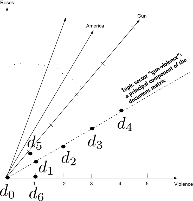
Figure 4.1 Document descriptor space. Each word in the vocabulary corresponds to a separate dimension. Dots show projections of document feature vectors on the plane formed by the axes corresponding to the terms gun and violence.
In figure 4.1, all the points representing documents are concentrated near the 45-degree line, and the rest of the plane is unpopulated. Can we collapse the two axes defining that plane and replace them with the single line around which most data is concentrated? It turns out that yes, we can do this. Doing so reduces the number of dimensions in the data representation—we are replacing a pair of correlated dimensions with a single one—thereby simplifying the representation. This leads to lower storage costs and, more importantly, provides additional insights. We have effectively discovered a new topic called gun-violence from the documents.
as another example, consider a set of points in 3D, represented by coordinates X, Y, Z. If the Z coordinate is near zero for all the points, the data is concentrated around the X, Y plane. We can (and should) represent these points in two dimensions by projecting them onto the Z = 0 plane. Doing so approximates the positions of the points only slightly (they are projected onto a plane that they were close to in the first place). In a more realistic example, the data points may be clustered around an arbitrary plane in the 3D space (as opposed to the Z = 0 plane). We can still reduce the dimensionality of these data points to 2D by projecting on the plane they are close to.
In general, if a set of data points is distributed in a space so that the points are clustered around a lower-dimensional subspace within that space (such as a plane or line), we can project the points onto the subspace and perform a dimensionality reduction on the data. We effectively approximate the distances from the subspace with zero: since these distances are small by definition, the approximation is not too bad. Viewed another way, we eliminate smaller from-subspace variations and retain the larger in-subspace variations. The resulting representation is more compressed and also lends itself more easily to better analysis and insights as we have eliminated unimportant perturbations and are focusing on the main pattern.
These ideas form the basis of the technique called principal component analysis (PCA). It is one of the most important tools in the repertoire of a data scientist and machine learning practitioner. These ideas also underlie the latent semantic analysis (LSA) technique for document retrieval—a fundamental approach for solving natural language processing (NLP) problems in machine learning. This chapter is dedicated to studying a set of methods leading to PCA and LSA. We examine a basic document retrieval system along with Python code.
4.2 Quadratic forms and their minimization
Given a square symmetric matrix A, the scalar quantity Q = ![]() TA
TA![]() is called a quadratic form. These are seen in various situations in machine learning.
is called a quadratic form. These are seen in various situations in machine learning.
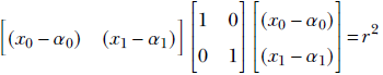
For instance, recall the equation for a circle that we learned in high school
(x0−α0)2 + (x1−α1)2 = r2
where the center of the circle is (α0, α1) and the radius is r. This equation can be rewritten as
If we denote the position vector ![]() as
as ![]() and the center of the circle as
and the center of the circle as ![]() as
as ![]() , the previous equation can be written compactly as
, the previous equation can be written compactly as
(![]() −
−![]() )TI(
)TI(![]() −
−![]() ) = r2
) = r2
Note that left hand side of this equation is a quadratic form. The original x0, x1-based equation only works for two dimensions. The matrix based equation is dimension agnostic: it represents a hypersphere in an arbitrary-dimensional space. For a two-dimensional space, the two equations become identical.
Now, consider the equation for an ellipse:
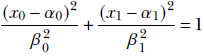
You can verify that this can be written compactly in matrix form as
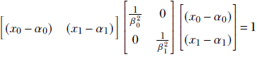
or, equivalently,
![]()
Equation 4.1
where 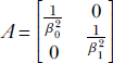 . Once again, the matrix representation is dimension independent. In other words, equation 4.1 represents a hyperellipsoid. Note that if the ellipse axes are aligned with the coordinate axes, matrix A is diagonal. If we rotate the coordinate system, each position vector is rotated by an orthogonal matrix R. Equation 4.1 is transformed as follows (we have used the rules for transposing the products of matrices from equation 2.10):
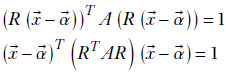
Replacing RTAR with A, we get the same equation as equation 4.1, but A is no longer a diagonal matrix.
For a generic ellipsoid with arbitrary axes, A has nonzero off-diagonal terms but is still symmetric. Thus, the multidimensional hyperellipsoid is represented by a quadratic form. The hypersphere is a special case of this.
Quadratic forms are also found in the second term of the multidimensional Taylor expansion shown in equation 3.8: ![]() is a quadratic form in the Hessian matrix. Another huge application of quadratic forms is PCA, which is so important that we devote a whole section to it section 4.4).
is a quadratic form in the Hessian matrix. Another huge application of quadratic forms is PCA, which is so important that we devote a whole section to it section 4.4).
4.2.1 Minimizing quadratic forms
An important question is, what choice of ![]() maximizes or minimizes the quadratic form? For instance, because the quadratic form is part of the multidimensional Taylor series, we need to minimize quadratic forms when we want to determine the best direction to move in to minimize the loss L(
maximizes or minimizes the quadratic form? For instance, because the quadratic form is part of the multidimensional Taylor series, we need to minimize quadratic forms when we want to determine the best direction to move in to minimize the loss L(![]() ). Later, we will see that this question also lies at the heart of PCA computation.
). Later, we will see that this question also lies at the heart of PCA computation.
If ![]() is a vector with arbitrary length, we can make Q arbitrarily big or small by simply changing the length of
is a vector with arbitrary length, we can make Q arbitrarily big or small by simply changing the length of ![]() . Consequently, optimizing Q with arbitrary length
. Consequently, optimizing Q with arbitrary length ![]() is not a very interesting problem: rather, we want to know which direction of
is not a very interesting problem: rather, we want to know which direction of ![]() optimizes Q. For the rest of this section, we discuss quadratic forms with unit vectors Q = x̂TAx̂ recall that x̂ denotes a unit-length vector satisfying x̂Tx̂ = ||x̂||2 = 1). Equivalently, we could use a different flavor, Q =
optimizes Q. For the rest of this section, we discuss quadratic forms with unit vectors Q = x̂TAx̂ recall that x̂ denotes a unit-length vector satisfying x̂Tx̂ = ||x̂||2 = 1). Equivalently, we could use a different flavor, Q = ![]() TA
TA![]() /
/![]() T
T![]() , but we will use the former expression here. We are essentially searching over all possible directions x̂, examining which direction minimizes Q = x̂TAx̂.
, but we will use the former expression here. We are essentially searching over all possible directions x̂, examining which direction minimizes Q = x̂TAx̂.
Using matrix diagonalization (section 2.15),
Q = x̂TAx̂ = x̂TSΛSTx̂
where S = [![]() 1
1 ![]() 2 …
2 … ![]() n] is the matrix with eigenvectors of A as its columns and Λ is a diagonal matrix with the eigenvalues of A on the diagonal and 0 everywhere else. Substituting
n] is the matrix with eigenvectors of A as its columns and Λ is a diagonal matrix with the eigenvalues of A on the diagonal and 0 everywhere else. Substituting
ŷ = STx̂
we get
Q = x̂TAx̂ = x̂TSΛSTx̂ = ŷTΛŷ
Equation 4.2
Note that since A is symmetric, its eigenvectors are orthogonal. This implies that S is an orthogonal matrix: that is, STS = SST = I. Recall from section 2.14.2.1 that for an orthogonal matrix S, the transformation STx̂ is length preserving. Consequently, ŷ = STx̂ is a unit-length vector. To be precise,
||ŷ||2 = ||STx̂||2 = (STx̂)T(STx̂) = x̂TSSTx̂ = x̂Tx̂ = 1 since SST = I
So, expanding the right-hand side of equation 4.2, we get
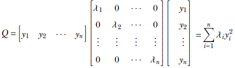
Equation 4.3
We can assume that the eigenvalues are sorted in decreasing order of magnitude (if not, we can always renumber them).
Consider this lemma (small proof): The quantity Σin= 1 λi yi2, where Σin= 1 yi2 = 1 and λ1 ≥ λ2 ≥ ⋯ λn, attains its maximum value when y1 = 1, y2 = ⋯ yn = 0.
An intuitive proof follows. If possible, let that the maximum value occur at some other value of ŷ. We are constrained by the fact that ŷ is an unit vector, so we must maintain Σin= 1 yi2 = 1.
In particular, none of the elements of ŷ can exceed 1. If we reduce the first term from 1 to a smaller value, say √1-ϵ, some other element(s) must go up by an equivalent amount to compensate (i.e., maintain the unit length property). Accordingly, suppose the hypothesized ŷ maximizing Q is given by
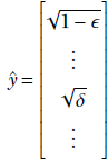
where δ > 0.
What happens if we transfer the entire mass from the later term to the first term so that
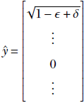
Doing this does not alter the length of ŷ as the sum of the squares of the first and the other term remains 1 − ϵ + δ. But the value of Q = Σin= 1 λi2 is higher in the second case (where ![]() 1 has been beefed up at the expense of another term), since λ1(1−ϵ + δ) > λ1(1−ϵ) + λjδ for any j > 1 (since, λ1 > λ2⋯ by assumption). Thus, whenever we have less than 1 in the first term and greater than zero in some other term, we can increase Q without losing the unit length property of ŷ by transferring the entire mass to the first term.
1 has been beefed up at the expense of another term), since λ1(1−ϵ + δ) > λ1(1−ϵ) + λjδ for any j > 1 (since, λ1 > λ2⋯ by assumption). Thus, whenever we have less than 1 in the first term and greater than zero in some other term, we can increase Q without losing the unit length property of ŷ by transferring the entire mass to the first term.
This means to maximize the right hand side of equation 4.3, we must have 1 as the first element (corresponding to the largest eigenvalue) of the unit vector ŷ and zeros everywhere else. Anything else violates the condition that the corresponding quadratic form Q = Σin= 1 λi2 is a maximum.
Thus we have established that the maximum of Q occurs at  . The corresponding x̂ = Sŷ =
 ![]() 1 - the eigenvector corresponding to the largest eigenvalue of A.
1 - the eigenvector corresponding to the largest eigenvalue of A.
Thus, the quadratic form Q = x̂TAx̂ attains its maximum when x̂ is along the eigenvector corresponding to the largest eigenvalue of A. The corresponding maximum Q is equal to the largest eigenvalue of A. Similarly, the minimum of the quadratic form occurs when x̂ is along the eigenvector corresponding to the smallest eigenvalue.
As stated above, many machine learning problems boil down to minimizing a quadratic form. We will study a few of them in later sections.
4.2.2 Symmetric positive (semi)definite matrices
A square symmetric n × n matrix A is positive semidefinite if and only if
![]() TA
TA![]() ≥ 0 ∀
≥ 0 ∀![]() ∈ ℝn
∈ ℝn
In other words, a positive semidefinite matrix yields a non-negative quadratic form with all n × 1 vectors ![]() . If we disallow the equality, we get symmetric positive definite matrices. Thus a square symmetric n × n matrix A is positive definite if and only if
. If we disallow the equality, we get symmetric positive definite matrices. Thus a square symmetric n × n matrix A is positive definite if and only if
![]() TA
TA![]() > 0 ∀
> 0 ∀![]() ∈ ℝn
∈ ℝn
From equations 4.2 and 4.3, Q is positive or zero if all λis are positive or zero (since the ![]() i2s are non-negative). Hence, symmetric positive (semi)definiteness is equivalent to the condition that all eigenvalues of the matrix are greater than (or equal to) zero.
i2s are non-negative). Hence, symmetric positive (semi)definiteness is equivalent to the condition that all eigenvalues of the matrix are greater than (or equal to) zero.
4.3 Spectral and Frobenius norms of a matrix
A vector is an entity with a magnitude and direction. The norm ||![]() || of a vector
|| of a vector ![]() represents its magnitude. Is there an equivalent notion for matrices? The answer is yes, and we will study two such ideas.
represents its magnitude. Is there an equivalent notion for matrices? The answer is yes, and we will study two such ideas.
4.3.1 Spectral norms
In section 2.5.4, we saw that the length (aka magnitude) of a vector ![]() is ||
is ||![]() || =
|| = ![]() T
T![]() . Is there an equivalent notion of magnitude for a matrix A?
. Is there an equivalent notion of magnitude for a matrix A?
Well, a matrix can be viewed as an amplifier of a vector. The matrix A amplifies the vector ![]() to
to ![]() = A
= A![]() . So we can take the maximum possible value of ||A
. So we can take the maximum possible value of ||A![]() || over all possible
|| over all possible ![]() ; that is a measure for the magnitude of A. Of course, if we consider arbitrary-length vectors, we can make
; that is a measure for the magnitude of A. Of course, if we consider arbitrary-length vectors, we can make ![]() arbitrarily large by simply scaling
arbitrarily large by simply scaling ![]() for any A. That is uninteresting. Rather, we want to examine which direction of
for any A. That is uninteresting. Rather, we want to examine which direction of ![]() is amplified most and by how much.
is amplified most and by how much.
We examine this question with unit vectors x̂: what is the maximum (or minimum) value of ||Ax̂||, and what direction x̂ materializes it? The quantity
![]()
is known as the spectral norm of the matrix A. Note that A![]() is a vector and ||A
is a vector and ||A![]() ||2 is its length. (We will sometimes drop the subscript 2 and denote the spectral norm as ||A||.)
||2 is its length. (We will sometimes drop the subscript 2 and denote the spectral norm as ||A||.)
Now consider the vector Ax̂. Its magnitude is
||Ax̂|| = (Ax̂)T(Ax̂) = x̂TATAx̂
This is a quadratic form. From section 4.2, we know it will be maximized (minimized) when x̂ s aligned with the largest smallest) eigenvalue of ATA. Thus the spectral norm is given by the largest eigenvalue of ATA
![]()
Equation 4.4
where σ1 is the largest eigenvalue of ATA. It is also (the square of) the largest singular value of A. We will see σ1 again in section 4.5, when we study singular value decomposition (SVD).
4.3.2 Frobenius norms
An alternative measure for the magnitude of a matrix is the Frobenius norm, defined as
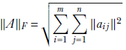
Equation 4.5
In other words, it is the root mean square of all the matrix elements.
It can be proved that the Frobenius norm is equal to the root mean square of the sum of all the singular values (eigenvalues of ATA) of the matrix
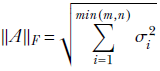
Equation 4.6
4.4 Principal component analysis
Suppose we have a set of numbers, X = {x(0), x(1),⋯, x(n)}. We want to get a sense of how tightly packed these points are. In other words, we want to measure the spread of these numbers. Figure 4.2 shows such a distribution.
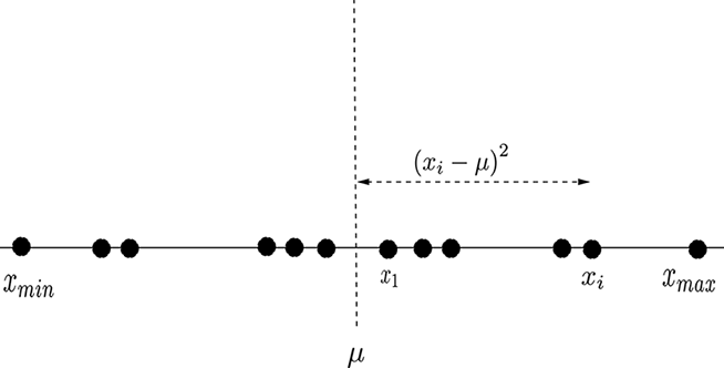
Figure 4.2 A 1D distribution of points. The distance between extreme points is not a fair representation of the spread of points: the distribution is not uniform, and the extreme points are far from the others. Most points are within a more tightly packed region.
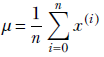
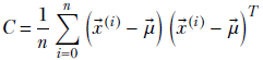
Note that the points need not be uniformly distributed. In particular, the extreme points (xmax, xmin) may be far from most other points (as in figure 4.2). Thus, (xmax– xmin)/(n+1) is not a fair representation of the average spread of points here. Most points are within a more tightly packed region. The statistically sensible way to obtain the spread is to first obtain the mean:
Then obtain the average distance of the numbers from the mean:
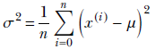
(If we want to, we can take the square root and use σ, but it is often not necessary to incur that extra computational burden). This scalar quantity, σ, is a good measure of the mean packing density or spread of the points in 1D. You may recognize that the previous equation is nothing but the famous variance formula from statistics. Can we extend the notion to higher-dimensional data?
Let’s first examine the idea in two dimensions. As usual, we name our coordinate axes X0, X1, and so on, instead of X, Y, to facilitate the extension to multiple dimensions. An individual 2D data point is denoted  . The dataset is {
![]() (0),
(0), ![]() (1), ⋯,
(1), ⋯, ![]() (n)}.
(n)}.
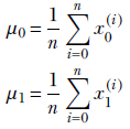
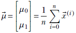
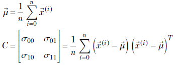
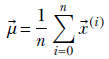
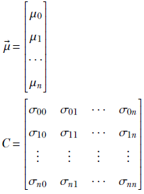
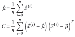
The mean is straightforward. Instead of one means, we have two:
Thus we now have a mean vector:
Now let’s do the variance. The immediate problem we face is that there are infinite possible directions in the 2D plane. We can measure variance along any of them, and it will be different for each choice. We can, of course, find the variance along the X0 and X1 axes:
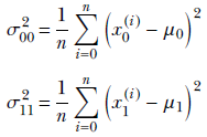
σ00 and σ11 tells us the variance along only one of the axes X0 and X1, respectively. But in general, there will be joint variation along both axes. To deal with joint variation, let’s introduce a cross term:
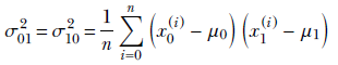
These equations can be written compactly in matrix vector notation:
NOTE In the expression for C, we are not taking the dot product of the vectors (![]() (i)−
(i)−![]() ) and (
) and (![]() (i)−
(i)−![]() ). The dot product would be (
). The dot product would be (![]() (i)−
(i)−![]() )T(
)T(![]() (i)−
(i)−![]() ). Here, the second element of the product is transposed, not the first. Consequently, the result is a matrix. The dot product would yield a scalar.)
). Here, the second element of the product is transposed, not the first. Consequently, the result is a matrix. The dot product would yield a scalar.)
The previous equations are general, meaning they can be extended to any dimension. To be precise, given a set of n multidimensional data points X = {![]() (0),
(0), ![]() (1),⋯,
(1),⋯, ![]() (n)}, we can define
(n)}, we can define
Equation 4.7
Equation 4.8
Note how the mean has become a vector (it was a scalar for 1D data) and the scalar variance of 1D, σ, has become a matrix C. This matrix is called the covariance matrix. The (n+1)-dimensional mean and covariance matrix can also be defined a
Equation 4.9
where
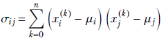
Equation 4.10
For i = j, σii is essentially the variance of the data along the ith dimension. Thus the diagonal elements of matrix C contain the variance along the coordinate axes. Off-diagonal elements correspond to cross-covariances.
NOTE Equations 4.8 and 4.9 are equivalent.
4.4.1 Direction of maximum spread
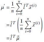
What is the direction of maximum spread/variance? Let’s first consider an arbitrary direction specified by the unit vector l̂. Recalling that the component of any vector along a direction is yielded by the dot product of the vector with the unit direction vector, the components of the data points along l̂ are given by
X ′ = {l̂ T![]() (0), l̂ T
(0), l̂ T![]() (1),⋯, l̂ T
(1),⋯, l̂ T![]() (n)}
(n)}
NOTE Remember figure 2.8b, which showed that the component of one vector along another is given by the dot product between them? l̂ T![]() (i) are dot products and hence scalar values.
(i) are dot products and hence scalar values.
The spread along direction l̂ is given by the variance of the scalar values in X ′. The mean of the values in X ′ is given by
and the variance is
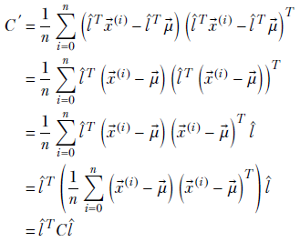
Note that C ′ = l̂ TCl̂ is the variance of the data components along the direction l̂. As such, it represents the spread of the data along that direction. What is the direction l̂ along which this spread l̂ TCl̂ is maximal? It is the direction l̂ that maximizes C ′ = l̂ TCl̂. This maximizing direction can be identified using the quadratic form optimization technique we discussed in 4.2. Applying that, we have the following results:
-
Variance is maximal when l̂ is along the eigenvector corresponding to the largest eigenvalue of the covariance matrix C. This direction is called the first principal axis of the multidimensional data.
-
The components of the data vectors along the principal axis are known as first principal components.
-
The value of the variance along the first principal axis, given by the corresponding eigenvalue of the covariance matrix, is called the first principal value.
-
The second principal axis is the eigenvector of the covariance matrix corresponding to the second largest eigenvalue of the covariance matrix. Second principal components and values are defined likewise.
-
The principal axes are orthogonal to each other because they are eigenvectors of the symmetric covariance matrix.
What is the practical significance of PCA? Why would we like to know the direction along which the spread is maximum for a point distribution? Sections 4.4.2 through 4.4.5 are devoted to answering this question.
4.4.2 PCA and dimensionality reduction
In section 4.1, we saw that when data points are clustered around a lower-dimensional subspace, it is beneficial to project them onto the subspace and reduce the dimensionality of the data representation. The dimensionally reduced data is more compactly representable and more amenable to deriving insights and analysis. In the particular case where the data points are clustered around a straight line or hyperplane, PCA can be used to generate a lower-dimensional data representation by getting rid of the principal components corresponding to relatively small principal values. The technique is agnostic to the dimensionality of the data. The line or hyperplane can be anywhere in the space, with arbitrary orientation.
(a) Dimensionality reduction from 2D to 1D
(b) Dimensionality reduction from 3D to 2D
Figure 4.3 Dimensionality reduction via PCA. Original data points are shown with filled little circles, and hollow circles represent lower-dimensional representations.
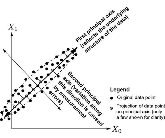
For instance, consider the 2D distribution shown in figure 4.3a. Here, the data is 2D and plotted on a plane, but the main spread of the data is along a 1D line shown by the thick two-arrowed line in the figure). There is very little spread in the direction orthogonal to that line (indicated by the little perpendiculars from the data points to the line in the figure). PCA reveals this internal structure. There are two principal values because the data is 2D), but one of them is much smaller than the other: this reveals that dimensionality reduction is possible. The principal axis corresponding to the larger principal value is along the line of maximum spread. The small perturbations along the other principal axis can be eliminated with little loss of information. Replacing each data point with its projection on the first principal axis converts the 2D dataset into a 1D dataset, brings out the true underlying pattern in the data (straight line), eliminates noise (little perpendiculars), and reduces storage costs.
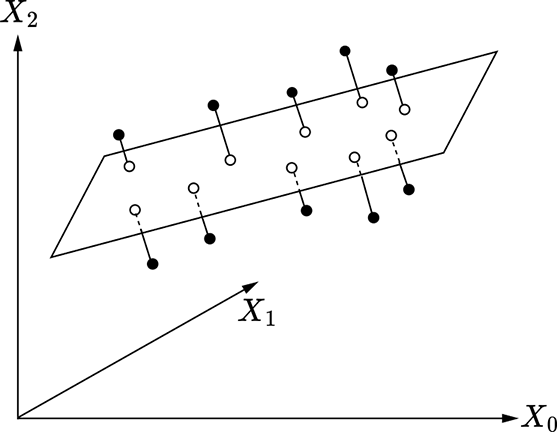
In figure 4.3b, the data is 3D, but the data points are clustered around a plane in 3D space (shown as the rectangle in the figure). The main spread of the data is along the plane, while the spread in the direction normal to that plane (shown with little perpendiculars from data points to the plane) is small. PCA reveals this: there are three principal values (because the data is 3D), but one of them is much smaller than the other two, revealing that dimensionality reduction is possible. The principal axis corresponding to the small principal value is normal to the plane. We can ignore these perturbations (perpendiculars in figure 4.3b) with little loss of information. This is equivalent to projecting the data onto the plane formed by the first two principal axes. Doing so brings out the underlying data pattern (plane), eliminates noise (little perpendiculars), and reduces storage costs.
4.4.3 PyTorch code: PCA and dimensionality reduction
In this section, we provide a PyTorch code sample for PCA computation in listing 4.1. Then we provide PyTorch code for applying PCA on a correlated dataset and an uncorrelated dataset in listings 4.2 and 4.3, respectively. The results are plotted in figure 4.4.
(a) PCA on correlated data
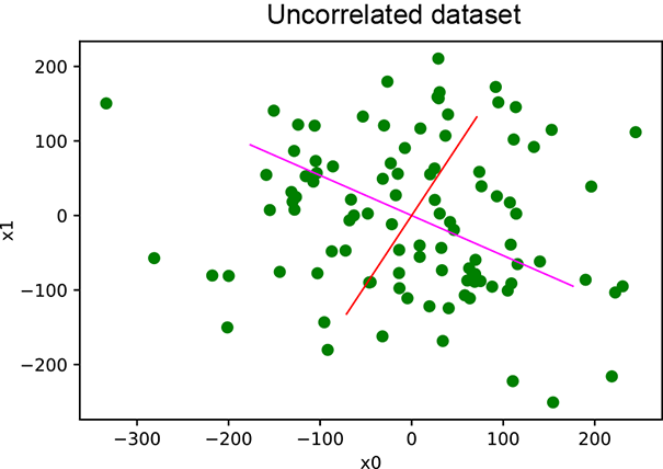
(b) PCA on uncorrelated data
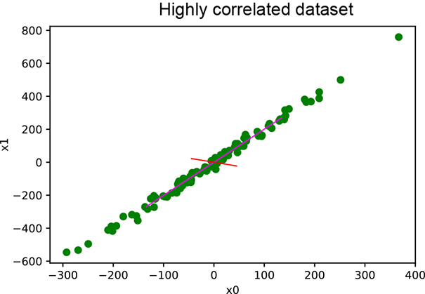
Figure 4.4 PCA results. In (a), the data points are around the straight line y = 2x. Consequently, one principal value is much larger than the other, indicating that dimensionality reduction will work. In (b), both principal values are large. Dimensionality reduction will not work.
NOTE The complete PyTorch code for this section is available at http://mng.bz/aoYz in the form of fully functional and executable Jupyter notebooks.
Listing 4.1 PCA computation
def pca(X):                                  ①
    covariance_matrix = torch.cov(X.T)
    l, e = torch.linalg.eig(covariance_matrix)
    return l, e
① Returns principal values and vectors
NOTE Fully functional code for the PCA computation in listing 4.1 is available at http://mng.bz/DRYR.
x_0 = torch.normal(0, 100, (N,))              ①

x_1 = 2 * x_0 + torch.normal(0, 20, (N,))     ②

  ③
X = torch.column_stack((x_0, x_1))

  ④
principal_values, principal_vectors = pca(X)  ⑤

X_proj = torch.matmul(X, first_princpal_vec)  ⑥
① Random feature vector
② Correlated feature vector + minor noise
③ Data matrix spread mostly along y = 2x
④ One large principal value and one small
⑤ First principal vector along y = 2x
⑥ Dimensionality reduction by projecting on the first principal vector
The output is as follows:
Principal values are: [62.6133, 48991.0469]
First Principal Vector is: [-0.44, -0.89]
NOTE Fully functional code for the PCA computation in listing 4.2 is available at http://mng.bz/gojl.
x_0 = torch.normal(0, 100, (N,))
x_1 = torch.normal(0, 100, (N,))             ①
X = torch.column_stack((x_0, x_1))

principal_values, principal_vectors = pca(X) ②
① Random uncorrelated feature-vector pair
② Principal values close to each other. The spread of the data points is comparable in both directions.
Here is the output:
Principal values are [ 9736.4033, 7876.6592]
NOTE Fully functional code for the PCA computation in listing 4.3 is available at http://mng.bz/e5Kz.
4.4.4 Limitations of PCA
PCA assumes that the underlying pattern is linear in nature. Where this is not true, PCA will not capture the correct underlying pattern. This is illustrated schematically in figure 4.5a and via experimental results from listing 4.3. Figure 4.5b shows the results of running listing 4.4, where we synthetically generate non-linearly correlated data and perform PCA. The straight line at the base shows the first principal axis. Projecting data on this axis results in a large error in the data positions (loss of information). Linear PCA will not do well.
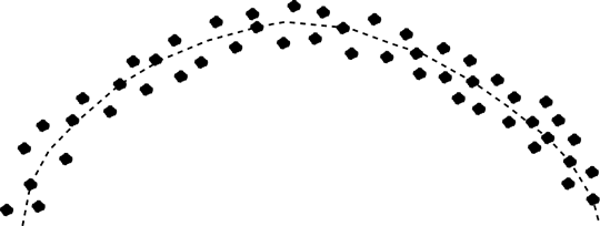
(a) Schematic 2D data distribution with a curved underlying pattern
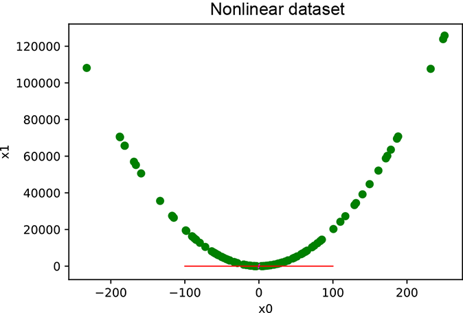
(b) PCA results on synthetic (computer generated) non-linearly correlated data. The line at the base shows the first principal axis.
Figure 4.5 Non-linearly correlated data. The points are distributed around a curve as opposed to a straight line. It is impossible to find a straight line such that all points are near it.
x_0 = torch.normal(0, 100, (N,))
x_1 = 2 * (x_0 ** 2) + torch.normal(0, 5, (N,))
X = torch.column_stack((x_0, x_1))

principal_values, principal_vectors = pca(X) ①
① Principal vectors fail to capture the underlying distribution.
The output is as follows:
Principal values are [9.3440e+03, 5.3373e+08]
Mean loss in information: 68.0108526887 - high
4.4.5 PCA and data compression
If we want to represent a large multidimensional dataset within a fixed byte budget, what information can we can get rid of with the least loss of accuracy? Clearly, the answer is the principal components along the smaller principal values—getting rid of them actually helps, as described in section 4.4.2. To compress data, we often perform PCA and then replace the data points with their projections on first few principal axes; doing so reduces the number of data components to store. This is the underlying principle in JPEG 98 image compression techniques.
4.5 Singular value decomposition
Singular value decomposition (SVD) may be the most important linear algebraic tool in machine learning. Among other things, PCA and LSA implementations are built based on SVD. We illustrate the basic idea in this section.
NOTE There are several slightly different forms of SVD. We have chosen the one that seems intuitively simplest.
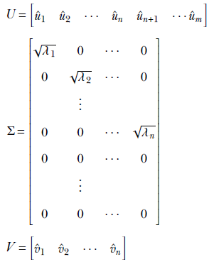
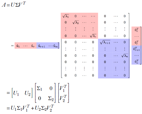
The SVD theorem states that any matrix A, singular or nonsingular, rectangular or square, can be decomposed as the product of three matrices
A = UΣVT
Equation 4.11
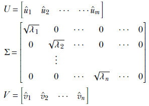
where (assuming that the matrix A is m × n)
-
Σ is an m × n diagonal matrix. Its diagonal elements contain the square roots of the eigenvalues of ATA. These are also known as the singular values of A. The singular values appear in decreasing order in the diagonal of Σ.
-
V is an n × n orthogonal matrix containing eigenvectors of ATA in its columns.
-
U is an m × m orthogonal matrix containing eigenvectors of AAT in its columns.
4.5.1 Informal proof of the SVD theorem
We will provide an informal proof of the SVD theorem through a series of lemmas. Going through these will provide additional insights.
Lemma 1
ATA is symmetric positive semidefinite. Its eigenvalues—aka singular values—are non-negative. Its eigenvectors—aka singular vectors—are orthogonal.
Proof of lemma 1
Let’s say A has m rows and n columns. Then ATA is an n × n square matrix
(ATA)T = AT(AT)T = ATA
which proves that ATA is symmetric. Also, for any ![]() ,
,
![]() TATA
TATA![]() = (A
= (A![]() )T(A
)T(A![]() ) = ||A
) = ||A![]() ||2 > 0
||2 > 0
which, as per section 4.2.2, proves that the matrix ATA is symmetric and positive semidefinite. Hence, its eigenvalues are all positive or zero.
We proved in section 2.13 that symmetric matrices have orthogonal eigenvectors. That proves that singular vectors are orthogonal.
Let (λi, v̂1), for i ∈ [1, n] be the set of eigenvalue, eigenvector pairs of ATA—aka the singular value, singular vector pair of A. Note that without loss of generality, we can assume λ1 ≥ λ2 ≥ ⋯ λn because if not, we can always renumber the eigenvalues and eigenvectors).
Now, by definition,
ATAv̂i = λiv̂i ∀i ∈ [1, n]
From lemma 1, singular vectors are orthogonal, and hence
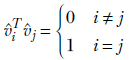
Equation 4.12
Note that v̂is are unit vectors (that is why we are using the hat sign as opposed to the overhead arrow). As described in section 2.13, eigenvectors remain eigenvectors if we change their length. We are free to choose any length for eigenvectors as long as we choose it consistently. We are choosing unit-length eigenvectors here.
Lemma 2
AAT is symmetric positive semidefinite. Its eigenvalues are non-negative and eigenvectors are orthogonal.
Proof of lemma 2
(AAT)T = (AT)TAT = AAT
Also,
![]() TAAT
TAAT![]() = (AT
= (AT![]() )T(AT
)T(AT![]() ) = ||(AT
) = ||(AT![]() )|| ≥ 0
)|| ≥ 0
and so on.
Lemma 3
1/√λi ⋅ Av̂1, ∀i ∈ [1, n] is a set of orthogonal unit vectors.
Proof of lemma 3
Let’s take the dot product of a pair of these vectors:
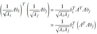
Since λj, v̂j are eigenvalue, eigenvector pairs of ATA, the previous equation can be rewritten as
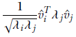
which, using equation 4.12, can be rewritten as
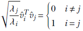
Lemma 4
If (λi, v̂i) is an eigenvalue, eigenvector pair of ATA, then λi, ûi = 1/√λi ⋅ Av̂i is an eigenvalue, eigenvector pair of AAT.
Proof of lemma 4
Given
ATAv̂i = λiv̂i
left-multiplying both sides of the equation by A, we get
AATAv̂i = λi Av̂i
AAT(Av̂i) = λi (Av̂i)
Substituting ![]() i = Av̂i in the last equation, we get
i = Av̂i in the last equation, we get
AAT![]() i = λi
i = λi![]() i
i
which proves that ![]() i = Av̂i is an eigenvector of AAT with λi as a corresponding eigenvalue. Multiplying by 1/√λi converts it into a unit vector as per lemma 3. This completes the proof of the lemma.
i = Av̂i is an eigenvector of AAT with λi as a corresponding eigenvalue. Multiplying by 1/√λi converts it into a unit vector as per lemma 3. This completes the proof of the lemma.
4.5.2 Proof of the SVD theorem
Now we are ready to examine the proof of the SVD theorem.
Case 1: More rows than columns in A
If m, the number of rows in A, is greater than or equal to n, the number of columns in A, we define
Note the following:
-
From lemma 1, we know that the eigenvalues of ATA are positive. This makes the square roots, √λis, real.
-
U is an m × m orthogonal matrix whose columns are the eigenvectors of AAT. Since, AAT is m × m, it has m eigenvalues and eigenvectors. The first n of them are û1 = 1/√λ1 ⋅ Av̂1, û2 = 1/√λ2 ⋅ Av̂2, … , ûn = 1/√λi ⋅ Av̂n from lemma 4, we know these are eigenvectors of AAT). In this case, by our initial assumption, n < m. Thus AAT has (m − n) more eigenvectors, ûn + 1, ⋯ ûm.
-
V is an n × n orthogonal matrix with the eigenvectors of ATA that is, v̂1, v̂2, ⋯, v̂n) as its columns.
Consider the matrix product UΣ. From basic matrix multiplication rules (section 2.5, we can see that
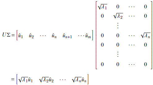
Note that the last columns of U, ûn + 1, ⋯, ûm, are multiplied by all zeros in Σ and vanishing. Thus,
The later columns of U—those named with us—fail to survive because they are multiplied by the zeros at the bottom of Σ.
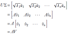
Thus we have proved that
AV = UΣ
Then
AVVT = UΣVT
Since V is orthogonal, VVT = I. Hence
A = UΣVT
which completes the proof of the singular value theorem.
Case 2: Fewer rows than columns in A
If m, the number of rows in A, is less than or equal to n, the number of columns in A, we have
The proof follows along similar lines.
4.5.3 Applying SVD: PCA computation
We will illustrate the idea first with a toy dataset. Consider a 3D dataset with five points. We use a superscript to denote the index of the data instance and a subscript to denote the component. Thus the ith data instance vector is denoted as [x0(i) x1(i) x2(i)]. We denote the entire data set with a matrix in which each feature instance appears as a row vector. The data matrix is
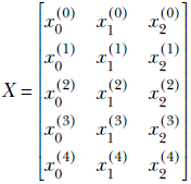
We will assume that the data is already mean-subtracted. Now examine the matrix product XTX, using ordinary rules of matrix multiplication:
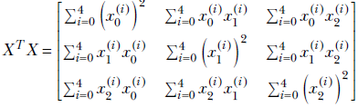
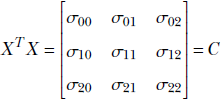
Thus XTX is the covariance matrix of the dataset X. This holds for arbitrary dimensions and arbitrary feature instance counts.
If we create a data matrix X with each data instance forming a row, XTX ields the covariance matrix of the dataset. The eigenvalues and eigenvectors of this matrix are the principal components. Hence, performing SVD on X yields PCA of the data (assuming prior mean subtraction).
4.5.4 Applying SVD: Solving arbitrary linear systems
A linear system is a system of simultaneous linear equations
A![]() =
= ![]()
We first encountered a linear system in section 2.12. It is possible to use matrix inversion to solve such a system:
![]() = A-1
= A-1![]()
However, solving a linear system with matrix inversion is undesirable for many reasons. To begin with, it is numerically unstable. The matrix inverse contains the determinant of the matrix in its denominator. If the determinant is near zero, the inverse will contain very large numbers. Minor noise in ![]() will be multiplied by these large numbers and cause large errors in the computed solution
will be multiplied by these large numbers and cause large errors in the computed solution ![]() . In this case, the inverse-based solution can be very inaccurate. Furthermore, the determinant can be zero: this can happen when one row of the matrix is a linear combination of others, indicating that we have fewer equations than we think. And what if the matrix is not square to begin with? This can happen when we have more equations than unknowns overdetermined system) or fewer equations than unknowns underdetermined system). In these cases, the inverse is not computable, and the system cannot be solved fully.
. In this case, the inverse-based solution can be very inaccurate. Furthermore, the determinant can be zero: this can happen when one row of the matrix is a linear combination of others, indicating that we have fewer equations than we think. And what if the matrix is not square to begin with? This can happen when we have more equations than unknowns overdetermined system) or fewer equations than unknowns underdetermined system). In these cases, the inverse is not computable, and the system cannot be solved fully.
Even in these cases, we would like to obtain a solution that is the best approximation in some sense; and in the case of a square matrix, we would like to get the exact solution. How do we do this? Answer: we use SVD. The steps are as follows:
-
A
 =
=  can be rewritten as U(ΣVT) = . We then solve U
 1 = . This can be easily done using orthogonality of U, as 1 = UT.
 -
Now we have Σ(VT
) = 1 Solve Σ2 = 1. This can be easily done because for any diagonal matrix 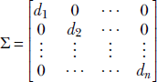 we can easily compute
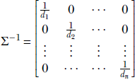
Hence,
2 = Σ−11. -
Now we have VT
= 2. This too can be solved easily using the orthogonality of V: = V2
Thus we have solved for ![]() without inverting the matrix A:
without inverting the matrix A:
-
For invertible square matrices A, this method yields the same solution as the matrix-inverse-based method.
-
For nonsquare matrices, this boils down to the Moore-Penrose inverse and yields the best-effort solution.
4.5.5 Rank of a matrix
In section 2.12, we studied linear systems of equations. Such a system can be represented in matrix-vector form:
A![]() =
= ![]()
Each row of A and ![]() contributes one equation. If we have as many independent equations as unknowns, the system is solvable. This is the simplest case; matrix A is square and invertible. det(A) is nonzero, and A−1 exists.
contributes one equation. If we have as many independent equations as unknowns, the system is solvable. This is the simplest case; matrix A is square and invertible. det(A) is nonzero, and A−1 exists.
Sometimes the situation is misleading. Consider the following system:
Although there are three rows and apparently three equations, the equations are not independent. For instance, the third equation can be obtained by adding the first two. We really have only two equations, not three. We say this linear system is degenerate. All of the following statements are true for such a system A![]() =
= ![]() :
:
-
The linear system is degenerate.
-
det(A) = 0.
-
A−1 cannot be computed, and A is not invertible.
-
Rows of A are linearly dependent. There exists a linear combination of the rows that sum to zero. For example, in the previous example,
 0 + 1 − 2 = 0.
 -
At least one of the singular values of A (eigenvalues of ATA) is zero. The number of linearly independent rows is equal to the number of nonzero eigenvalues.
The number of linearly independent rows in a matrix is called its rank. It can be proved that a matrix has as many nonzero singular values as its rank. It can also be proved that the number of linearly independent columns in a matrix matches the number of linearly independent rows. Hence, rank can also be defined as the number of linearly independent columns in a matrix.
A nonsquare rectangular matrix with m rows and n columns has a rank r = min(m, n). Such matrices are never invertible. We usually resort to SVD to solve them.
A square matrix with n rows and n columns is invertible nonzero determinant) if and only if it has rank n. Such a matrix is said to have full rank. Full-rank matrices are invertible. They can be solved via matrix inverse computation, but inverse computation is not always numerically stable. SVD can be applied here as well, with good numerical properties.
Non-full-rank matrices are degenerate. So, rank is a measure of the non-degeneracy of the matrix.
4.5.6 PyTorch code for solving linear systems with SVD
The listings in this section show a PyTorch-based implementation of SVD and demonstrate an application that solves a linear system via SVD.
Listing 4.5 Solving an invertible linear system with matrix inversion and SVD
A = torch.tensor([[1, 2, 1], [2, 2, 3], [1, 3, 3]]).float()
b = torch.tensor([8, 15, 16]).float()      ①

x_0 = torch.matmul(torch.linalg.inv(A), b) ②

U, S, V_t = torch.linalg.svd(A)            ③

y1 = torch.matmul(U.T, b)                  ④

S_inv = torch.diag(1 / S)

y2 = torch.matmul(S_inv, y1)               ⑤

x_1 = torch.matmul(V_t.T, y2)              ⑥

assert torch.allclose(x_0, x_1)            ⑦
① Simple test linear system of equations
② Matrix inversion is numerically unstable; SVD is better.
③ A = USVT ⟹ A![]() =
= ![]() ≜ USVT
≜ USVT![]() =
= ![]()
④ Solves U![]() 1 =
1 = ![]() . Remember U−1 = UT as U is orthogonal.
. Remember U−1 = UT as U is orthogonal.
⑤ Solves S![]() 2 =
2 = ![]() 1. Remember S−1 is easy as S is diagonal.
1. Remember S−1 is easy as S is diagonal.
⑥ Solves VT ![]() =
= ![]() 2. Remember V−T = V as V is orthogonal.
2. Remember V−T = V as V is orthogonal.
⑦ The two solutions are the same.
Solution via inverse: [1.0, 2.0, 3.0]
Solution via SVD: [1.0, 2.0, 3.0]
Listing 4.6 Solving an overdetermined linear system by pseudo-inverse and SVD
A = torch.tensor([[0.11, 0.09], [0.01, 0.02],
              [0.98, 0.91], [0.12, 0.21],
              [0.98, 0.99], [0.85, 0.87],
              [0.03, 0.14], [0.55, 0.45],
              [0.49, 0.51], [0.99, 0.01],
              [0.02, 0.89], [0.31, 0.47],
              [0.55, 0.29], [0.87, 0.76],
              [0.63, 0.24]])                         ①
A = torch.column_stack((A, torch.ones(15)))
b = torch.tensor([-0.8, -0.97, 0.89, -0.67,
              0.97, 0.72, -0.83, 0.00,
              0.00, 0.00, -0.09, -0.22,
              -0.16, 0.63, 0.37])

x_0 = torch.matmul(torch.linalg.pinv(A), b)          ②

U, S, V_t = torch.linalg.svd(A, full_matrices=False) ③

y1 = torch.matmul(U.T, b)
S_inv = torch.diag(1 / S)
y2 = torch.matmul(S_inv, y1)
x_1 = torch.matmul(V_t.T, y2)


assert torch.allclose(x_0, x_1)                      ④
① Cat-brain dataset: nonsquare matrix
② Solution via pseudo-inverse
③ Solution via SVD
④ The two solutions are the same.
The output is as follows:
Solution via pseudo-inverse: [ 1.0766, 0.8976, -0.9582]
Solution via SVD: [ 1.0766, 0.8976, -0.9582]
Fully functional code for solving the SVD-based linear system can be found at http://mng.bz/OERn.
4.5.7 PyTorch code for PCA computation via SVD
The following listing demonstrates PCA computations using SVD.
Listing 4.7 Computing PCA directly and using SVD
  ①                ②               ③
principal_values, principal_vectors = pca(X) ④

X_mean = X - torch.mean(X, axis=0)

  ⑤
U, S, V_t = torch.linalg.svd(X_mean)         ⑥

V = V_t.T                                    ⑦
① Eigenvalues of the covariance matrix yield principal values.
② Eigenvectors of the covariance matrix yield principal vectors.
③ Direct PCA computation from a covariance matrix
④ Data matrix
⑤ Diagonal elements of matrix S yield principal values.
⑥ PCA from SVD
⑦ Columns of matrix V yield principal vectors.
The output is as follows:
Principal components obtained via PCA:
[[-0.44588404 -0.89509073]
 [-0.89509073 0.44588404]]
Principal components obtained via SVD:
[[-0.44588404 0.89509073]
 [-0.89509073 -0.44588404]]
4.5.8 Applying SVD: Best low-rank approximation of a matrix
Given a matrix A of some rank p, we sometimes want to approximate it with a matrix of lower rank r, where r < p. How do we obtain the best rank r approximation of A?
Motivation
Why would we want to do this? Well, consider a data matrix X as shown in section 4.5.3. As explained in section 4.4.2, we often want to eliminate small variances in the data (likely due to noise) and get the pattern underlying large variations. Replacing the data matrix with a lower-rank matrix often achieves this. However, we must bear in mind that this does not work when the underlying pattern is nonlinear (such as in figure 4.5a).
Approximation error
What do we mean by best approximation? The Frobenius norm can be taken as the magnitude of the matrix. Accordingly, given a matrix A and its rank r approximation Ar, the approximation error is e = ||A − Ar||F.
Method
To solidify our ideas, let’s consider an m × n matrix A. From section 4.5, we know it will have min(m, n) singular values. Let its rank be p ≤ min(m, n). We want to approximate this matrix with a rank r(<p) matrix.
Let’s rewrite the SVD expression. We will assume m > n. Also, as usual, we have the singular values sorted in decreasing order: λ1 ≥ λ2 ≥ λn. We will partition U, Σ, V:
It can be proved that U1Σ1V1T is a rank r matrix. Furthermore, it is the best rank r approximation of A.
4.6 Machine learning application: Document retrieval
We will now bring together several of the concepts we have discussed in this chapter with an illustrative toy example: the document retrieval problem we first encountered in section 2.1. Briefly recapping, we have a set of documents {d0,⋯, d6}. Given an incoming query phrase, we have to retrieve documents that match the query phrase. We will use the bag of words model: that is, our matching approach does not pay attention to where a word appears in a document; it simply pays attention to how many times the word appears in the document. Although this technique is not the most sophisticated, it is popular because of its conceptual simplicity.
Our documents are as follows:
-
d0: Roses are lovely. Nobody hates roses.
-
d1: Gun violence has reached epidemic proportions in America.
-
d2: The issue of gun violence is really over-hyped. One can find many instances of violence where no guns were involved.
-
d3: Guns are for violence prone people. Violence begets guns. Guns beget violence.
-
d4: I like guns but I hate violence. I have never been involved in violence. But I own many guns. Gun violence is incomprehensible to me. I do believe gun owners are the most anti violence people on the planet. He who never uses a gun will be prone to senseless violence.
-
d5: Guns were used in an armed robbery in San Francisco last night.
-
d6: Acts of violence usually involve a weapon.
4.6.1 Using TF-IDF and cosine similarity
Before discussing PCA, let’s look at some more elementary techniques for document retrieval. These are based on term frequency-inverse document frequency (TF-IDF) and cosine similarity.
Term frequency
Term frequency (TF) is defined as the number of occurrences of a particular term in a document. (In this context, note that in this book, we use term and word somewhat interchangeably.) In a slightly looser definition, any quantity proportional to the number of occurrences of the term is also known as term frequency. For example, the TF of the word gun in d0, d6 is 0, in d1 is 1, in d3 is 3, and so on. Note that we are being case independent. Also, singular/plural (gun and guns) and various flavors of the words originating from the same stem (such as violence and violent) are typically mapped to the same term.
Inverse document frequency
Certain terms, such as the, appear in pretty much all documents. These should be ignored during document retrieval. How do we down-weight them?
The IDF is obtained by inverting and then taking the absolute value of the logarithm of the fraction of all documents in which the term occurs. For terms that occur in most documents, the IDF weight is very low. It is high for relatively esoteric terms.
Document feature vectors
Each document is represented by a document feature vector. It has as many elements as the size of the vocabulary (that is, the number of distinct words over all the documents). Every word has a fixed index position in the vector. Given a specific document, the value at the index position corresponding to a specific word contains the TF of the corresponding word multiplied by that word’s IDF. Thus, every document is a point in a space that has as many dimensions as the vocabulary size. The coordinate value along a specific dimension is proportional to the number of times the word is repeated in the document, with a weigh-down factor for common words.
For real-life document retrieval systems like Google, this vector is extremely long. But not to worry: this vector is notional—it is never explicitly stored in the computer’s memory. We store a sparse version of the document feature vector: a list of unique words along with their TF×IDF scores.
Cosine similarity
In section 2.5.6.2, we saw that the dot product between two vectors measures the agreement between them. Given two vectors ![]() and
and ![]() , we know
, we know ![]() ⋅
⋅ ![]() = ||
= ||![]() || ||
|| ||![]() ||cos(θ), where the operator || ⋅ || implies the length of a vector and θ is the angle between the two vectors (see figure 2.7b). The cosine is at its maximum possible value, 1, when the vectors are pointing in the same direction and the angle between them is zero. It becomes progressively smaller as the angle between the vectors increases until the two vectors are perpendicular to each other and the cosine is zero, implying no correlation: the vectors are independent of each other.
||cos(θ), where the operator || ⋅ || implies the length of a vector and θ is the angle between the two vectors (see figure 2.7b). The cosine is at its maximum possible value, 1, when the vectors are pointing in the same direction and the angle between them is zero. It becomes progressively smaller as the angle between the vectors increases until the two vectors are perpendicular to each other and the cosine is zero, implying no correlation: the vectors are independent of each other.
The magnitude of the dot product is also proportional to the length of the two vectors. We do not want to use the full dot product as a measure of similarity between the vectors because two long vectors would have a high similarity score even if they were not aligned in direction. Rather, we want to use the cosine, defined as
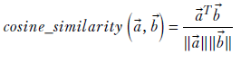
Equation 4.13
The cosine similarity between document vectors is a principled way of measuring the degree of term sharing between the documents. It is higher if many repeated words are shared between the two documents.
4.6.2 Latent semantic analysis
Cosine similarity and similar techniques suffer from a significant drawback. To see this, examine the cosine similarity between d5 and d6. It is zero. But it is obvious to a human that the documents are similar.
What went wrong? Answer: we are measuring only the direct overlap between terms in documents. The words gun and violence occur together in many of the other documents, indicating some degree of similarity between them. Hence, documents containing only gun have some similarity with documents containing only violence—but cosine similarity between document vectors does not look at such secondary evidence. This is the blind spot that LSA tries to overcome.
Words are known by the company they keep. That is, if terms appear together in many documents (like gun and violence in the previous examples), they are likely to share some semantic similarity. Such terms should be grouped together into a common pool of semantically similar terms. Such a pool is called a topic. Document similarity should be measured in terms of common topics rather than explicit common terms. We are particularly interested in topics that discriminate the documents in our corpus: that is, there should be a high variation in the degree to which different documents subscribe to the topic.
Geometrically, a topic is a subspace in the document feature space. In classical latent semantic analysis, we only look at linear subspaces, and a topic can be visualized as a direction or linear combination of directions (hyperplane) in the document feature space. In particular, any direction line in the space is a topic: it is a subspace representing a weighted combination of the coordinate axis directions, which means it is a weighted combination of vocabulary terms. We are, of course, interested in topics with high variance. These correspond to a direction along which the document vectors are well spread, which means the document vectors are well discriminated over this topic. We typically prune the set of topics, eliminating those with insufficient variance.
From this discussion, a mathematical definition of topic begins to emerge. Topics are principal components of the matrix of document vectors with individual document descriptor vectors along its rows. Measuring document similarity in terms of topic has the advantage that two documents may not have many exact words in common but may still have a common topic. This happens when they share words belonging to the same topic. Essentially, they share a lot of words that occur together in other documents. So even if the number of common words is low, we can have high document similarity.

Figure 4.6 Document vectors from our toy dataset d0, ⋯ d6. Each word in the vocabulary corresponds to a separate dimension. Dots show projections of document feature vectors on the plane formed by the axes corresponding to the terms gun(s) and violence.
For instance, in our toy document corpus, gun and violence are very correlated (both or neither is likely to occur in a document). Gun-violence emerges as a topic. If we express the document vector in terms of this topic instead of the individual words, we see similarities that otherwise would have escaped us. That is, we see latent semantic similarities. For instance, the cosine similarity between d5 and d6 is nonzero. This is the core idea of latent semantic analysis and is illustrated in figure 4.6.
Let’s revisit our example document-retrieval problem in light of topic extraction. The document matrix (with document vectors as rows) looks like table 4.1. Rows correspond to documents, and columns correspond to terms. Each cell contains the term frequency. The terms gun and violence occur an equal number of times in most documents, indicating clear correlation. Hence gun-violence is a topic. The principal components right eigenvectors) identify topics. As usual, we have omitted prepositions, conjunctions, commas, and so on. The overall steps are as follows (see listing 4.8 for the Python code):
-
Create a document term m × n. Its rows correspond to documents (m documents), and its columns correspond to terms (n terms).
-
Perform SVD on the matrix. This yields U, S, and V matrices. V is an n × n orthogonal matrix, and S is a diagonal matrix.
-
The columns of matrix V yield topics. These are principal vectors for the rows of X: that is, eigenvectors of XTX or, equivalently, the covariance matrix of X.
-
The successive elements of each topic vector (column in matrix V) tell us the contribution of corresponding terms to that topic. Each column is n × 1, depicting the contributions of the n terms in the system.
-
The diagonal elements of S tell us the weights (importance) of corresponding topics. These are the eigenvalues of XTX: that is, principal values of the row vectors of X.
-
Inspect the weights, and choose a cutoff. All topics below that weight are discarded—the corresponding columns of V are thrown away. This yields a matrix V with fewer columns but the same number of rows); these are the topic vectors of interest to us. We have reduced the dimensionality of the problem. If the number of retained topics is t, the reduced V is m × t.
-
By projecting (multiplying) the original matrix X of document terms to this new matrix V, we get an m × t matrix of document topics (it has same number of rows as X but fewer columns). This is the projection of X to the topic space: that is, a topic-based representation of the document vectors.
-
Rows of the document topic matrix will henceforth be taken as document representations. Document similarities will be computed by taking the cosine similarity of these rows rather than the rows of the original document term matrix. This cosine similarity, in the topic space, will capture many indirect connections that were not visible in the original input space.
Table 4.1 Document matrix for the toy example dataset
|
|
Violence |
Gun |
America |
⋯ |
Roses |
|---|---|---|---|---|---|
|
d0 |
0 |
0 |
0 |
⋯ |
2 |
|
d1 |
1 |
1 |
1 |
⋯ |
0 |
|
d2 |
2 |
2 |
0 |
⋯ |
0 |
|
d3 |
3 |
3 |
0 |
⋯ |
0 |
|
d4 |
5 |
5 |
0 |
⋯ |
0 |
|
d5 |
0 |
1 |
0 |
⋯ |
0 |
|
d6 |
1 |
0 |
0 |
⋯ |
0 |
4.6.3 PyTorch code to perform LSA
The following listing demonstrates how to compute the LSA for our toy dataset from table 4.1. Fully functional code for this section can be found at http://mng.bz/E2Gd.
Listing 4.8 Computing LSA
terms = ["violence", "gun", "america", "roses"]         ①
X = torch.tensor([[0, 0, 0, 2],
              [1, 1, 1, 0],
              [2, 2, 0, 0],
              [3, 3, 0, 0],
              [5, 5, 0, 0],
              [0, 1, 0, 0],
              [1, 0, 0, 0]]).float()                    ②

U, S, V_t = torch.linalg.svd(X)                         ③

V = V_t.T

rank = 1
U = U[:, :rank]
V = V[:, :rank]                                         ④

topic0_term_weights = list(zip(terms, V[:, 0]))         ⑤

def cosine_similarity(vec_1, vec_2):
    vec_1_norm = torch.linalg.norm(vec_1)
    vec_2_norm = torch.linalg.norm(vec_2)
    return torch.dot(vec_1, vec_2) / (vec_1_norm * vec_2_norm)

d5_d6_cosine_similarity = cosine_similarity(X[5], X[6]) ⑥

doc_topic_projection = torch.dot(X, V)
d5_d6_lsa_similarity = cosine_similarity(doc_topic_projection[5],
                                         doc_topic_projection[6])
① Considers only four terms for simplicity
② Document term matrix. Each row describes a document. Each column contains TF scores for one term. IDF is ignored for simplicity.
③ Performs SVD on the doc-term matrix. Columns of the resulting matrix V correspond to topics. These are eigenvectors of XTX: principal vectors of the doc-term matrix. A topic corresponds to the direction of maximum variance in the doc feature space.
④ S indicates the diagonal matrix of principal values. These signify topic weights (importance). We choose a cut-off and discard all topics below that weight (dimensionality reduction). Only the first few columns of V are retained. Principal values (topic weights) for this dataset are shown in the output. Only one topic is retained in this example.
⑤ Elements of the topic vector show the contributions of corresponding terms to the topic.
⑥ Cosine similarity in the feature space fails to capture d, d6 similarity. LSA succeeds.
The output is as follows:
Principal Values from S matrix: 8.89, 2.00, 1.00, 0.99
(Topic 0 has disproportionately high weight. We discard others)

topic0_term_weights (Topic zero is about "gun" and "violence"):
[
 ('violence', -0.706990662151775)
 ('gun', -0.7069906621517749)
 ('america', -0.018122010384881156)
 ('roses', 2.9413274625621952e-18)
]
Document 5, document 6 Cosine similarity in original space: 0.0
Document 5, document 6 Cosine similarity in topic space: 1.0
4.6.4 PyTorch code to compute LSA and SVD on a large dataset
Suppose we have a set of 500 documents over a vocabulary of 3 terms. This is an unrealistically short vocabulary, but it allows us to easily visualize the space of document vectors. Each document vector is a 3 × 1 vector, and there are 500 such vectors. Together they form a 500 × 3 data matrix X. In this dataset, the terms x0 and x1 are correlated: x0 occurs randomly between 0 and 100 times in a document, and x1 occurs twice as many times as x0 except for small random fluctuations. The third term’s frequency varies between 0 and 5. From section 4.6, we know that x0, x1 together form a single topic, while x2 by itself forms another topic. We expect a principal component along each topic.
Listing 4.9 creates the dataset, computes the SVD, plots the dataset, and shows the first two principal components. The third singular value is small compared to the first. We can ignore that dimension—it corresponds to the small random variation within the x0 − x1 topic. The singular values are printed out and also shown graphically along with the data points in figure 4.7.
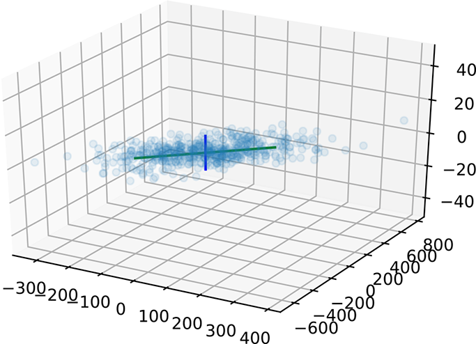
Figure 4.7 Latent semantic analysis. Note that the vertical axis line is actually much smaller than it appears to be in the diagram.
Listing 4.9 LSA using SVD
num_examples = 500
x0 = torch.normal(0, 100, (num_examples,)).round()
random_noise = torch.normal(0, 2, (num_examples,)).round()
x1 = 2*x0 + random_noise
x2 = torch.normal(0, 5, (num_examples,)).round()
X = torch.column_stack((x0, x1, x2))                       ①

                ②
U, S, V_t = torch.linalg.svd(X)                            ③
V = V_t.T                                                  ③
① 3D dataset: the first two axes are linearly correlated; the third axis has small near-zero random values.
② The third singular value is relatively small; we ignore it
③ The first two principal vectors represent topics. Projecting data points on them yields document descriptors in terms of the two topics.
Here is the output:
Singular values are: 4867.56982, 118.05858, 19.68604
Summary
In this chapter, we studied several linear algebraic tools used in machine learning and data science:
-
The direction (unit vector) that maximizes (minimizes) the quadratic form x̂TAx̂ is the eigenvector corresponding to the largest (smallest) eigenvalue of matrix A. The magnitude of the quadratic form when x̂ is along those directions is the largest (smallest) eigenvalue of A.
-
Given a set of points X = {
(0), (1), (2), ⋯, (n)} in an n + 1-dimensional space, we can define the mean vector and covariance matrix as
The variance along an arbitrary direction (unit vector) l̂ is l̂ TCl̂. This is a quadratic form. Consequently, the maximum (minimum) variance of a set of data points in multidimensional space occurs along the eigenvector corresponding to the largest (smallest) eigenvalue of the covariance matrix. This direction is called the first principal axis of the data. The subsequent eigenvectors, sorted in order of decreasing eigenvalues, are mutually orthogonal (perpendicular) and yield the subsequent direction of maximum variance. This technique is known as principal component analysis (PCA).
-
In many real-life cases, larger variances correspond to the true underlying pattern of the data, while smaller variances correspond to noise (such as measurement error). Projecting the data on the principal axes corresponding to the larger eigenvalues yields lower-dimensional data that is relatively noise-free. The projected data points also match the true underlying pattern more closely, yielding better insights. This is known as dimensionality reduction.
-
Singular value decomposition (SVD) allows us to decompose an arbitrary m × n matrix A as a product of three matrices: A = UΣVT, where U, V are orthogonal and Σ is diagonal. Matrix V has the eigenvectors of ATA as its columns. U has eigenvectors of AAT as columns. Σ has the eigenvalues of ATA sorted in decreasing order) in its diagonal.
-
SVD provides a numerically stable way to solve the linear system of equations A
= . In particular, for nonsquare matrices, it provides the closest approximations: that is, that minimizes ||A − ||. -
Given a dataset X whose rows are data vectors corresponding to individual instances and columns correspond to feature values, XTX ields the covariance matrix. Thus eigenvectors of XTX ield the data’s principal components. Since the SVD of X has eigenvectors of XTX as columns of the matrix V, SVD is an effective way to compute PCA.
-
When using machine learning data science for document retrieval, the bag-of-words model represents documents with document vectors that contain the term frequency (number of occurrences) of each term in the document.
-
TF-IDF is a cosine similarity technique for document matching and retrieval.
-
Latent semantic analysis (LSA) does topic modeling: we perform PCA on the document vectors to identify topics. Projecting document vectors onto topic axes allows LSA to see latent (indirect) similarities beyond the direct overlapping of terms.