7 Fine-tuning to follow instructions
This chapter covers
- The instruction fine-tuning process of LLMs
- Preparing a dataset for supervised instruction fine-tuning
- Organizing instruction data in training batches
- Loading a pretrained LLM and fine-tuning it to follow human instructions
- Extracting LLM-generated instruction responses for evaluation
- Evaluating an instruction-fine-tuned LLM
Previously, we implemented the LLM architecture, carried out pretraining, and imported pretrained weights from external sources into our model. Then, we focused on fine-tuning our LLM for a specific classification task: distinguishing between spam and non-spam text messages. Now we’ll implement the process for fine-tuning an LLM to follow human instructions, as illustrated in figure 7.1. Instruction fine-tuning is one of the main techniques behind developing LLMs for chatbot applications, personal assistants, and other conversational tasks.
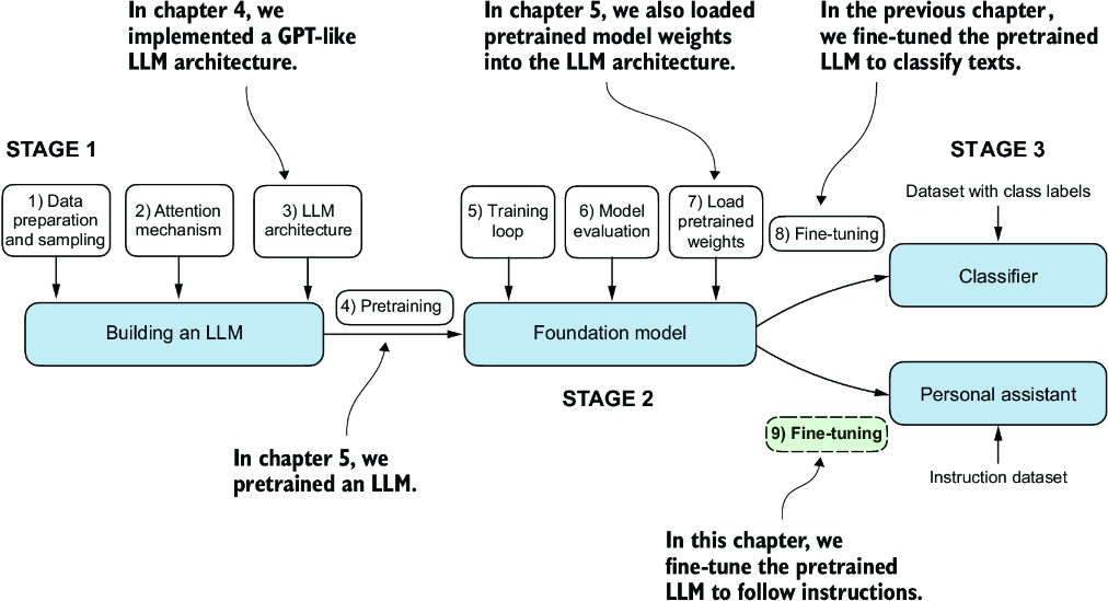
Figure 7.1 The three main stages of coding an LLM. This chapter focuses on step 9 of stage 3: fine-tuning a pretrained LLM to follow human instructions.
Figure 7.1 shows two main ways of fine-tuning an LLM: fine-tuning for classification (step 8) and fine-tuning an LLM to follow instructions (step 9). We implemented step 8 in chapter 6. Now we will fine-tune an LLM using an instruction dataset.
7.1 Introduction to instruction fine-tuning
We now know that pretraining an LLM involves a training procedure where it learns to generate one word at a time. The resulting pretrained LLM is capable of text completion, meaning it can finish sentences or write text paragraphs given a fragment as input. However, pretrained LLMs often struggle with specific instructions, such as “Fix the grammar in this text” or “Convert this text into passive voice.” Later, we will examine a concrete example where we load the pretrained LLM as the basis for instruction fine-tuning, also known as supervised instruction fine-tuning.
Here, we focus on improving the LLM’s ability to follow such instructions and generate a desired response, as illustrated in figure 7.2. Preparing the dataset is a key aspect of instruction fine-tuning. Then we’ll complete all the steps in the three stages of the instruction fine-tuning process, beginning with the dataset preparation, as shown in figure 7.3.
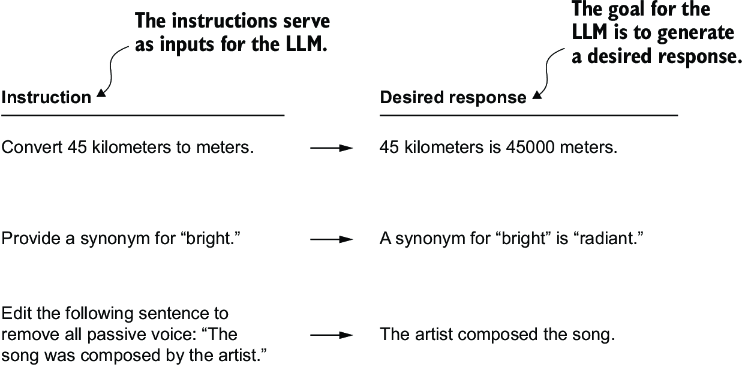
Figure 7.2 Examples of instructions that are processed by an LLM to generate desired responses
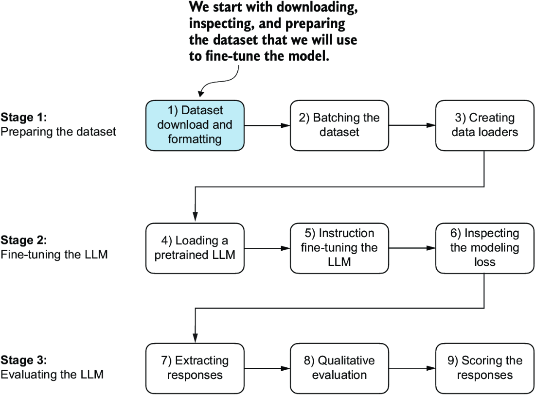
Figure 7.3 The three-stage process for instruction fine-tuning an LLM. Stage 1 involves dataset preparation, stage 2 focuses on model setup and fine-tuning, and stage 3 covers the evaluation of the model. We will begin with step 1 of stage 1: downloading and formatting the dataset.
7.2 Preparing a dataset for supervised instruction fine-tuning
Let’s download and format the instruction dataset for instruction fine-tuning a pretrained LLM. The dataset consists of 1,100 instruction–response pairs similar to those in figure 7.2. This dataset was created specifically for this book, but interested readers can find alternative, publicly available instruction datasets in appendix B.
The following code implements and executes a function to download this dataset, which is a relatively small file (only 204 KB) in JSON format. JSON, or JavaScript Object Notation, mirrors the structure of Python dictionaries, providing a simple structure for data interchange that is both human readable and machine friendly.
Listing 7.1 Downloading the dataset
import json
import os
import urllib

def download_and_load_file(file_path, url):
    if not os.path.exists(file_path):
        with urllib.request.urlopen(url) as response:
            text_data = response.read().decode("utf-8")
        with open(file_path, "w", encoding="utf-8") as file:
            file.write(text_data)
    else:                                                #1
        with open(file_path, "r", encoding="utf-8") as file:
            text_data = file.read()
    with open(file_path, "r") as file:
        data = json.load(file)
    return data

file_path = "instruction-data.json"
url = (
    "https://raw.githubusercontent.com/rasbt/LLMs-from-scratch"
    "/main/ch07/01_main-chapter-code/instruction-data.json"
)


data = download_and_load_file(file_path, url)
print("Number of entries:", len(data))
The output of executing the preceding code is
Number of entries: 1100
The data list that we loaded from the JSON file contains the 1,100 entries of the instruction dataset. Let’s print one of the entries to see how each entry is structured:
print("Example entry:\n", data[50])
The content of the example entry is
Example entry:
 {'instruction': 'Identify the correct spelling of the following word.',
  'input': 'Ocassion', 'output': "The correct spelling is 'Occasion.'"}
As we can see, the example entries are Python dictionary objects containing an 'instruction', 'input', and 'output'. Let’s take a look at another example:
print("Another example entry:\n", data[999])
Based on the contents of this entry, the 'input' field may occasionally be empty:
Another example entry:
 {'instruction': "What is an antonym of 'complicated'?",
  'input': '',
  'output': "An antonym of 'complicated' is 'simple'."}
Instruction fine-tuning involves training a model on a dataset where the input-output pairs, like those we extracted from the JSON file, are explicitly provided. There are various methods to format these entries for LLMs. Figure 7.4 illustrates two different example formats, often referred to as prompt styles, used in the training of notable LLMs such as Alpaca and Phi-3.
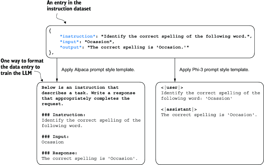
Figure 7.4 Comparison of prompt styles for instruction fine-tuning in LLMs. The Alpaca style (left) uses a structured format with defined sections for instruction, input, and response, while the Phi-3 style (right) employs a simpler format with designated <|user|> and <|assistant|> tokens.
Alpaca was one of the early LLMs to publicly detail its instruction fine-tuning process. Phi-3, developed by Microsoft, is included to demonstrate the diversity in prompt styles. The rest of this chapter uses the Alpaca prompt style since it is one of the most popular ones, largely because it helped define the original approach to fine-tuning.
Let’s define a format_input function that we can use to convert the entries in the data list into the Alpaca-style input format.
Listing 7.2 Implementing the prompt formatting function
def format_input(entry):
    instruction_text = (
        f"Below is an instruction that describes a task. "
        f"Write a response that appropriately completes the request."
        f"\n\\n### Instruction:\\n{entry['instruction']}"
    )

    input_text = (
        f"\n\\n### Input:\\n{entry['input']}" if entry["input"] else ""
    )
    return instruction_text + input_text
This format_input function takes a dictionary entry as input and constructs a formatted string. Let’s test it to dataset entry data[50], which we looked at earlier:
model_input = format_input(data[50])
desired_response = f"\n\\n### Response:\\n{data[50]['output']}"
print(model_input + desired_response)
The formatted input looks like as follows:
Below is an instruction that describes a task. Write a response that
appropriately completes the request.

### Instruction:
Identify the correct spelling of the following word.

### Input:
Ocassion

### Response:
The correct spelling is 'Occasion.'
Note that the format_input skips the optional ### Input: section if the 'input' field is empty, which we can test out by applying the format_input function to entry data[999] that we inspected earlier:
model_input = format_input(data[999])
desired_response = f"\n\\n### Response:\\n{data[999]['output']}"
print(model_input + desired_response)
The output shows that entries with an empty 'input' field don’t contain an ### Input: section in the formatted input:
Below is an instruction that describes a task. Write a response that
appropriately completes the request.

### Instruction:
What is an antonym of 'complicated'?

### Response:
An antonym of 'complicated' is 'simple'.
Before we move on to setting up the PyTorch data loaders in the next section, let’s divide the dataset into training, validation, and test sets analogous to what we have done with the spam classification dataset in the previous chapter. The following listing shows how we calculate the portions.
Listing 7.3 Partitioning the dataset
train_portion = int(len(data) * 0.85)    #1
test_portion = int(len(data) * 0.1)            #2
val_portion = len(data) - train_portion - test_portion    #3

train_data = data[:train_portion]
test_data = data[train_portion:train_portion + test_portion]
val_data = data[train_portion + test_portion:]

print("Training set length:", len(train_data))
print("Validation set length:", len(val_data))
print("Test set length:", len(test_data))
This partitioning results in the following dataset sizes:
Training set length: 935
Validation set length: 55
Test set length: 110
Having successfully downloaded and partitioned the dataset and gained a clear understanding of the dataset prompt formatting, we are now ready for the core implementation of the instruction fine-tuning process. Next, we focus on developing the method for constructing the training batches for fine-tuning the LLM.
7.3 Organizing data into training batches
As we progress into the implementation phase of our instruction fine-tuning process, the next step, illustrated in figure 7.5, focuses on constructing the training batches effectively. This involves defining a method that will ensure our model receives the formatted training data during the fine-tuning process.
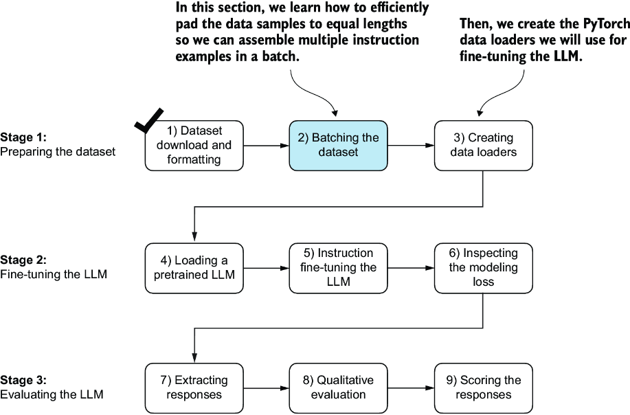
Figure 7.5 The three-stage process for instruction fine-tuning an LLM. Next, we look at step 2 of stage 1: assembling the training batches.
In the previous chapter, the training batches were created automatically by the PyTorch DataLoader class, which employs a default collate function to combine lists of samples into batches. A collate function is responsible for taking a list of individual data samples and merging them into a single batch that can be processed efficiently by the model during training.
However, the batching process for instruction fine-tuning is a bit more involved and requires us to create our own custom collate function that we will later plug into the DataLoader. We implement this custom collate function to handle the specific requirements and formatting of our instruction fine-tuning dataset.
Let’s tackle the batching process in several steps, including coding the custom collate function, as illustrated in figure 7.6. First, to implement steps 2.1 and 2.2, we code an InstructionDataset class that applies format_input and pretokenizes all inputs in the dataset, similar to the SpamDataset in chapter 6. This two-step process, detailed in figure 7.7, is implemented in the __init__ constructor method of the InstructionDataset.
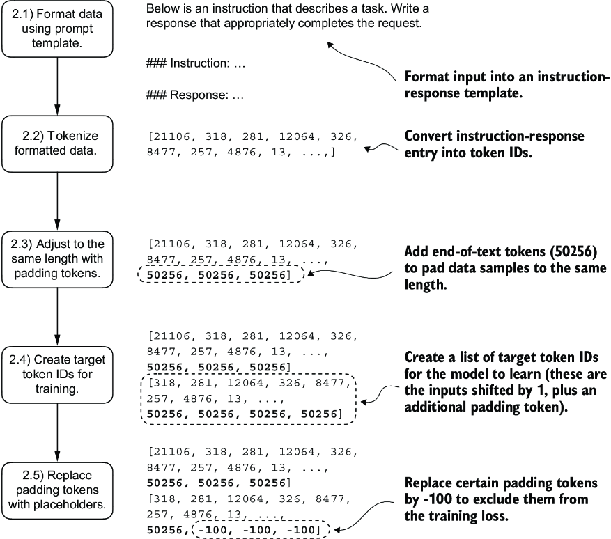
Figure 7.6 The five substeps involved in implementing the batching process: (2.1) applying the prompt template, (2.2) using tokenization from previous chapters, (2.3) adding padding tokens, (2.4) creating target token IDs, and (2.5) replacing -100 placeholder tokens to mask padding tokens in the loss function.
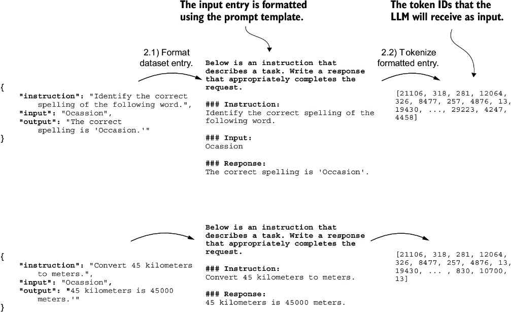
Figure 7.7 The first two steps involved in implementing the batching process. Entries are first formatted using a specific prompt template (2.1) and then tokenized (2.2), resulting in a sequence of token IDs that the model can process.
Listing 7.4 Implementing an instruction dataset class
import torch
from torch.utils.data import Dataset

class InstructionDataset(Dataset):
    def __init__(self, data, tokenizer):
        self.data = data
        self.encoded_texts = []
        for entry in data:         #1
            instruction_plus_input = format_input(entry)
            response_text = f"\n\\n### Response:\\n{entry['output']}"
            full_text = instruction_plus_input + response_text
            self.encoded_texts.append(
                tokenizer.encode(full_text)
            )

    def __getitem__(self, index):
        return self.encoded_texts[index]

    def __len__(self):
        return len(self.data)
Similar to the approach used for classification fine-tuning, we want to accelerate training by collecting multiple training examples in a batch, which necessitates padding all inputs to a similar length. As with classification fine-tuning, we use the <|endoftext|> token as a padding token.
Instead of appending the <|endoftext|> tokens to the text inputs, we can append the token ID corresponding to <|endoftext|> to the pretokenized inputs directly. We can use the tokenizer’s .encode method on an <|endoftext|> token to remind us which token ID we should use:
import tiktoken
tokenizer = tiktoken.get_encoding("gpt2")
print(tokenizer.encode("<|endoftext|>", allowed_special={"<|endoftext|>"}))
The resulting token ID is 50256.
Moving on to step 2.3 of the process (see figure 7.6), we adopt a more sophisticated approach by developing a custom collate function that we can pass to the data loader. This custom collate function pads the training examples in each batch to the same length while allowing different batches to have different lengths, as demonstrated in figure 7.8. This approach minimizes unnecessary padding by only extending sequences to match the longest one in each batch, not the whole dataset.
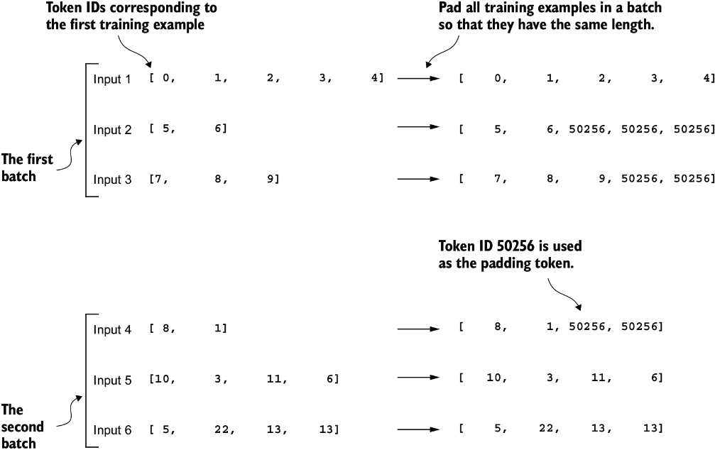
Figure 7.8 The padding of training examples in batches using token ID 50256 to ensure uniform length within each batch. Each batch may have different lengths, as shown by the first and second.
We can implement the padding process with a custom collate function:
def custom_collate_draft_1(
    batch,
    pad_token_id=50256,
    device="cpu"
):
    batch_max_length = max(len(item)+1 for item in batch)   #1
    inputs_lst = []

    for item in batch:     #2
        new_item = item.copy()
        new_item += [pad_token_id]


        padded = (
            new_item + [pad_token_id] *
            (batch_max_length - len(new_item))
        )
        inputs = torch.tensor(padded[:-1])    #3
        inputs_lst.append(inputs)

    inputs_tensor = torch.stack(inputs_lst).to(device)     #4
    return inputs_tensor
The custom_collate_draft_1 we implemented is designed to be integrated into a PyTorch DataLoader, but it can also function as a standalone tool. Here, we use it independently to test and verify that it operates as intended. Let’s try it on three different inputs that we want to assemble into a batch, where each example gets padded to the same length:
inputs_1 = [0, 1, 2, 3, 4]
inputs_2 = [5, 6]
inputs_3 = [7, 8, 9]
batch = (
    inputs_1,
    inputs_2,
    inputs_3
)
print(custom_collate_draft_1(batch))
The resulting batch looks like the following:
tensor([[    0,     1,     2,     3,     4],
        [    5,     6, 50256, 50256, 50256],
        [    7,     8,     9, 50256, 50256]])
This output shows all inputs have been padded to the length of the longest input list, inputs_1, containing five token IDs.
We have just implemented our first custom collate function to create batches from lists of inputs. However, as we previously learned, we also need to create batches with the target token IDs corresponding to the batch of input IDs. These target IDs, as shown in figure 7.9, are crucial because they represent what we want the model to generate and what we need during training to calculate the loss for the weight updates. That is, we modify our custom collate function to return the target token IDs in addition to the input token IDs.
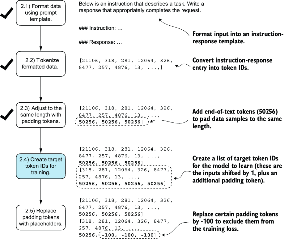
Figure 7.9 The five substeps involved in implementing the batching process. We are now focusing on step 2.4, the creation of target token IDs. This step is essential as it enables the model to learn and predict the tokens it needs to generate.
Similar to the process we used to pretrain an LLM, the target token IDs match the input token IDs but are shifted one position to the right. This setup, as shown in figure 7.10, allows the LLM to learn how to predict the next token in a sequence.
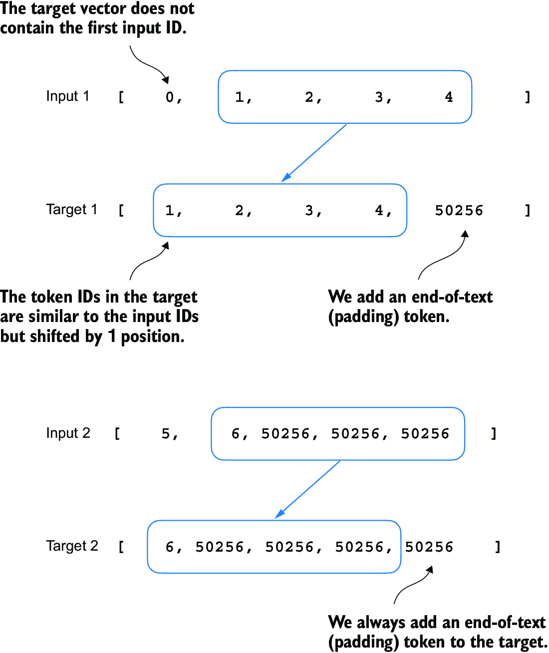
Figure 7.10 The input and target token alignment used in the instruction fine-tuning process of an LLM. For each input sequence, the corresponding target sequence is created by shifting the token IDs one position to the right, omitting the first token of the input, and appending an end-of-text token.
The following updated collate function generates the target token IDs from the input token IDs:
def custom_collate_draft_2(
    batch,
    pad_token_id=50256,
    device="cpu"
):
    batch_max_length = max(len(item)+1 for item in batch)
    inputs_lst, targets_lst = [], []

    for item in batch:
        new_item = item.copy()
        new_item += [pad_token_id]

        padded = (
            new_item + [pad_token_id] *
            (batch_max_length - len(new_item))
        )
        inputs = torch.tensor(padded[:-1])     #1
        targets = torch.tensor(padded[1:])    #2
        inputs_lst.append(inputs)
        targets_lst.append(targets)

    inputs_tensor = torch.stack(inputs_lst).to(device)
    targets_tensor = torch.stack(targets_lst).to(device)
    return inputs_tensor, targets_tensor

inputs, targets = custom_collate_draft_2(batch)
print(inputs)
print(targets)
Applied to the example batch consisting of three input lists we defined earlier, the new custom_collate_draft_2 function now returns the input and the target batch:
tensor([[    0,     1,     2,     3,     4],    #1
        [    5,     6, 50256, 50256, 50256],
        [    7,     8,     9, 50256, 50256]])
tensor([[    1,     2,     3,     4, 50256],   #2
        [    6, 50256, 50256, 50256, 50256],
        [    8,     9, 50256, 50256, 50256]])
In the next step, we assign a -100 placeholder value to all padding tokens, as highlighted in figure 7.11. This special value allows us to exclude these padding tokens from contributing to the training loss calculation, ensuring that only meaningful data influences model learning. We will discuss this process in more detail after we implement this modification. (When fine-tuning for classification, we did not have to worry about this since we only trained the model based on the last output token.)
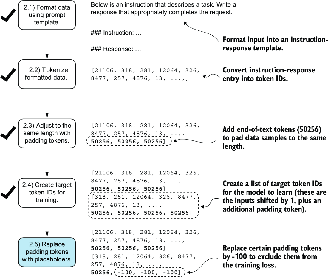
Figure 7.11 The five substeps involved in implementing the batching process. After creating the target sequence by shifting token IDs one position to the right and appending an end-of-text token, in step 2.5, we replace the end-of-text padding tokens with a placeholder value (-100).
However, note that we retain one end-of-text token, ID 50256, in the target list, as depicted in figure 7.12. Retaining it allows the LLM to learn when to generate an end-of-text token in response to instructions, which we use as an indicator that the generated response is complete.
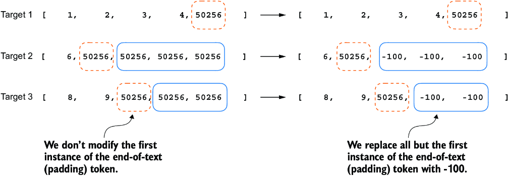
Figure 7.12 Step 2.4 in the token replacement process in the target batch for the training data preparation. We replace all but the first instance of the end-of-text token, which we use as padding, with the placeholder value -100, while keeping the initial end-of-text token in each target sequence.
In the following listing, we modify our custom collate function to replace tokens with ID 50256 with -100 in the target lists. Additionally, we introduce an allowed_ max_length parameter to optionally limit the length of the samples. This adjustment will be useful if you plan to work with your own datasets that exceed the 1,024-token context size supported by the GPT-2 model.
Listing 7.5 Implementing a custom batch collate function
def custom_collate_fn(
    batch,
    pad_token_id=50256,
    ignore_index=-100,
    allowed_max_length=None,
    device="cpu"
):
    batch_max_length = max(len(item)+1 for item in batch)
    inputs_lst, targets_lst = [], []

    for item in batch:
        new_item = item.copy()
        new_item += [pad_token_id]


        padded = (                               #1
            new_item + [pad_token_id] *          #1
            (batch_max_length - len(new_item))   #1
        )
        inputs = torch.tensor(padded[:-1])      #2
        targets = torch.tensor(padded[1:])     #3

        mask = targets == pad_token_id              #4
        indices = torch.nonzero(mask).squeeze()     #4
        if indices.numel() > 1:                     #4
            targets[indices[1:]] = ignore_index     #4

        if allowed_max_length is not None:
            inputs = inputs[:allowed_max_length]       #5
            targets = targets[:allowed_max_length]     #5

        inputs_lst.append(inputs)
        targets_lst.append(targets)

    inputs_tensor = torch.stack(inputs_lst).to(device)
    targets_tensor = torch.stack(targets_lst).to(device)
    return inputs_tensor, targets_tensor
Again, let’s try the collate function on the sample batch that we created earlier to check that it works as intended:
inputs, targets = custom_collate_fn(batch)
print(inputs)
print(targets)
The results are as follows, where the first tensor represents the inputs and the second tensor represents the targets:
tensor([[    0,     1,     2,     3,     4],
        [    5,     6, 50256, 50256, 50256],
        [    7,     8,     9, 50256, 50256]])
tensor([[    1,     2,     3,     4, 50256],
        [    6, 50256,  -100,  -100,  -100],
        [    8,     9, 50256,  -100,  -100]])
The modified collate function works as expected, altering the target list by inserting the token ID -100. What is the logic behind this adjustment? Let’s explore the underlying purpose of this modification.
For demonstration purposes, consider the following simple and self-contained example where each output logit corresponds to a potential token from the model’s vocabulary. Here’s how we might calculate the cross entropy loss (introduced in chapter 5) during training when the model predicts a sequence of tokens, which is similar to what we did when we pretrained the model and fine-tuned it for classification:
logits_1 = torch.tensor(
    [[-1.0, 1.0],     #1
     [-0.5, 1.5]]      #2
)
targets_1 = torch.tensor([0, 1]) # Correct token indices to generate
loss_1 = torch.nn.functional.cross_entropy(logits_1, targets_1)
print(loss_1)
The loss value calculated by the previous code is 1.1269:
tensor(1.1269)
As we would expect, adding an additional token ID affects the loss calculation:
logits_2 = torch.tensor(
    [[-1.0, 1.0],
     [-0.5, 1.5],
     [-0.5, 1.5]]      #1
)
targets_2 = torch.tensor([0, 1, 1])
loss_2 = torch.nn.functional.cross_entropy(logits_2, targets_2)
print(loss_2)
After adding the third token, the loss value is 0.7936.
So far, we have carried out some more or less obvious example calculations using the cross entropy loss function in PyTorch, the same loss function we used in the training functions for pretraining and fine-tuning for classification. Now let’s get to the interesting part and see what happens if we replace the third target token ID with -100:
targets_3 = torch.tensor([0, 1, -100])
loss_3 = torch.nn.functional.cross_entropy(logits_2, targets_3)
print(loss_3)
print("loss_1 == loss_3:", loss_1 == loss_3)
The resulting output is
tensor(1.1269)
loss_1 == loss_3: tensor(True)
The resulting loss on these three training examples is identical to the loss we calculated from the two training examples earlier. In other words, the cross entropy loss function ignored the third entry in the targets_3 vector, the token ID corresponding to -100. (Interested readers can try to replace the -100 value with another token ID that is not 0 or 1; it will result in an error.)
So what’s so special about -100 that it’s ignored by the cross entropy loss? The default setting of the cross entropy function in PyTorch is cross_entropy(..., ignore_index=-100). This means that it ignores targets labeled with -100. We take advantage of this ignore_index to ignore the additional end-of-text (padding) tokens that we used to pad the training examples to have the same length in each batch. However, we want to keep one 50256 (end-of-text) token ID in the targets because it helps the LLM to learn to generate end-of-text tokens, which we can use as an indicator that a response is complete.
In addition to masking out padding tokens, it is also common to mask out the target token IDs that correspond to the instruction, as illustrated in figure 7.13. By masking out the LLM’s target token IDs corresponding to the instruction, the cross entropy loss is only computed for the generated response target IDs. Thus, the model is trained to focus on generating accurate responses rather than memorizing instructions, which can help reduce overfitting.
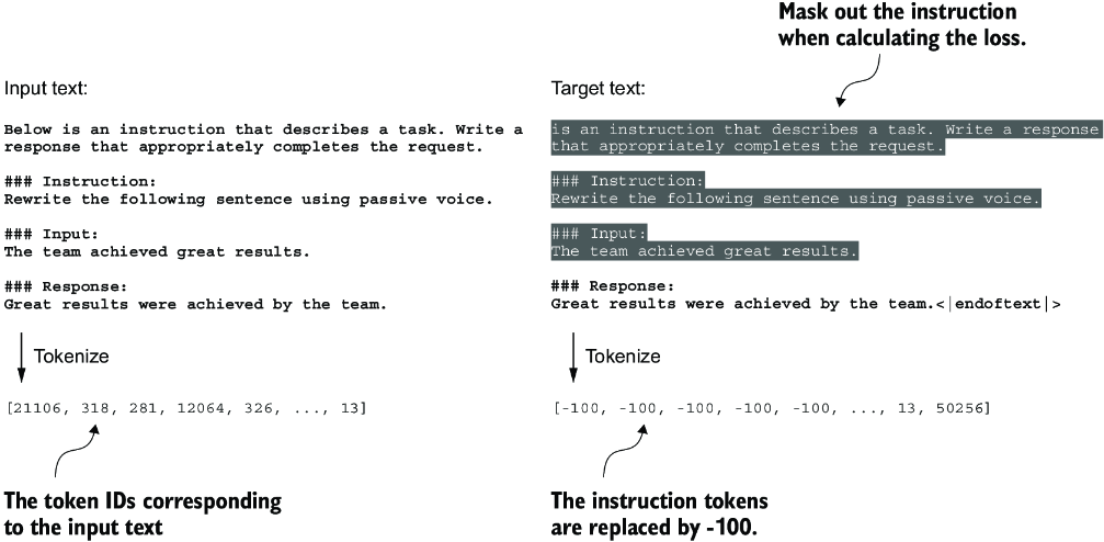
Figure 7.13 Left: The formatted input text we tokenize and then feed to the LLM during training. Right: The target text we prepare for the LLM where we can optionally mask out the instruction section, which means replacing the corresponding token IDs with the -100 ignore_index value.
As of this writing, researchers are divided on whether masking the instructions is universally beneficial during instruction fine-tuning. For instance, the 2024 paper by Shi et al., “Instruction Tuning With Loss Over Instructions” (https://arxiv.org/abs/2405.14394), demonstrated that not masking the instructions benefits the LLM performance (see appendix B for more details). Here, we will not apply masking and leave it as an optional exercise for interested readers.
7.4 Creating data loaders for an instruction dataset
We have completed several stages to implement an InstructionDataset class and a custom_collate_fn function for the instruction dataset. As shown in figure 7.14, we are ready to reap the fruits of our labor by simply plugging both InstructionDataset objects and the custom_collate_fn function into PyTorch data loaders. These loaders will automatically shuffle and organize the batches for the LLM instruction fine-tuning process.
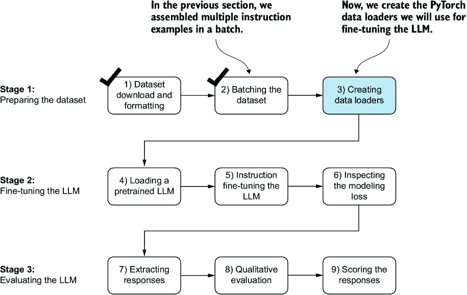
Figure 7.14 The three-stage process for instruction fine-tuning an LLM. Thus far, we have prepared the dataset and implemented a custom collate function to batch the instruction dataset. Now, we can create and apply the data loaders to the training, validation, and test sets needed for the LLM instruction fine-tuning and evaluation.
Before we implement the data loader creation step, we have to briefly talk about the device setting of the custom_collate_fn. The custom_collate_fn includes code to move the input and target tensors (for example, torch.stack(inputs_lst).to (device)) to a specified device, which can be either "cpu" or "cuda" (for NVIDIA GPUs) or, optionally, "mps" for Macs with Apple Silicon chips.
Note Using an "mps" device may result in numerical differences compared to the contents of this chapter, as Apple Silicon support in PyTorch is still experimental.
Previously, we moved the data onto the target device (for example, the GPU memory when device="cuda") in the main training loop. Having this as part of the collate function offers the advantage of performing this device transfer process as a background process outside the training loop, preventing it from blocking the GPU during model training.
The following code initializes the device variable:
device = torch.device("cuda" if torch.cuda.is_available() else "cpu")
# if torch.backends.mps.is_available():   #1
#     device = torch.device("mps")"
print("Device:", device)
This will either print "Device: cpu" or "Device: cuda", depending on your machine.
Next, to reuse the chosen device setting in custom_collate_fn when we plug it into the PyTorch DataLoader class, we use the partial function from Python’s functools standard library to create a new version of the function with the device argument prefilled. Additionally, we set the allowed_max_length to 1024, which truncates the data to the maximum context length supported by the GPT-2 model, which we will fine-tune later:
from functools import partial

customized_collate_fn = partial(
    custom_collate_fn,
    device=device,
    allowed_max_length=1024
)
Next, we can set up the data loaders as we did previously, but this time, we will use our custom collate function for the batching process.
Listing 7.6 Initializing the data loaders
from torch.utils.data import DataLoader

num_workers = 0      #1
batch_size = 8

torch.manual_seed(123)

train_dataset = InstructionDataset(train_data, tokenizer)
train_loader = DataLoader(
    train_dataset,
    batch_size=batch_size,
    collate_fn=customized_collate_fn,
    shuffle=True,
    drop_last=True,
    num_workers=num_workers
)

val_dataset = InstructionDataset(val_data, tokenizer)
val_loader = DataLoader(
    val_dataset,
    batch_size=batch_size,
    collate_fn=customized_collate_fn,
    shuffle=False,
    drop_last=False,
    num_workers=num_workers
)

test_dataset = InstructionDataset(test_data, tokenizer)
test_loader = DataLoader(
    test_dataset,
    batch_size=batch_size,
    collate_fn=customized_collate_fn,
    shuffle=False,
    drop_last=False,
    num_workers=num_workers
)
Let’s examine the dimensions of the input and target batches generated by the training loader:
print("Train loader:")
for inputs, targets in train_loader:
    print(inputs.shape, targets.shape)
The output is as follows (truncated to conserve space):
Train loader:
torch.Size([8, 61]) torch.Size([8, 61])
torch.Size([8, 76]) torch.Size([8, 76])
torch.Size([8, 73]) torch.Size([8, 73])
...
torch.Size([8, 74]) torch.Size([8, 74])
torch.Size([8, 69]) torch.Size([8, 69])
This output shows that the first input and target batch have dimensions 8 × 61, where 8 represents the batch size and 61 is the number of tokens in each training example in this batch. The second input and target batch have a different number of tokens—for instance, 76. Thanks to our custom collate function, the data loader is able to create batches of different lengths. In the next section, we load a pretrained LLM that we can then fine-tune with this data loader.
7.5 Loading a pretrained LLM
We have spent a lot of time preparing the dataset for instruction fine-tuning, which is a key aspect of the supervised fine-tuning process. Many other aspects are the same as in pretraining, allowing us to reuse much of the code from earlier chapters.
Before beginning instruction fine-tuning, we must first load a pretrained GPT model that we want to fine-tune (see figure 7.15), a process we have undertaken previously. However, instead of using the smallest 124-million-parameter model as before, we load the medium-sized model with 355 million parameters. The reason for this choice is that the 124-million-parameter model is too limited in capacity to achieve satisfactory results via instruction fine-tuning. Specifically, smaller models lack the necessary capacity to learn and retain the intricate patterns and nuanced behaviors required for high-quality instruction-following tasks.
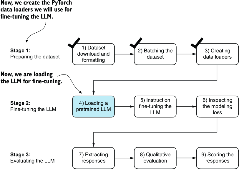
Figure 7.15 The three-stage process for instruction fine-tuning an LLM. After the dataset preparation, the process of fine-tuning an LLM for instruction-following begins with loading a pretrained LLM, which serves as the foundation for subsequent training.
Loading our pretrained models requires the same code as when we pretrained the data (section 5.5) and fine-tuned it for classification (section 6.4), except that we now specify "gpt2-medium (355M)" instead of "gpt2-small (124M)".
Note Executing this code will initiate the download of the medium-sized GPT model, which has a storage requirement of approximately 1.42 gigabytes. This is roughly three times larger than the storage space needed for the small model.
Listing 7.7 Loading the pretrained model
from gpt_download import download_and_load_gpt2
from chapter04 import GPTModel
from chapter05 import load_weights_into_gpt

BASE_CONFIG = {
    "vocab_size": 50257,     # Vocabulary size
    "context_length": 1024,  # Context length
    "drop_rate": 0.0,        # Dropout rate
    "qkv_bias": True         # Query-key-value bias
}

model_configs = {
    "gpt2-small (124M)": {"emb_dim": 768, "n_layers": 12, "n_heads": 12},
    "gpt2-medium (355M)": {"emb_dim": 1024, "n_layers": 24, "n_heads": 16},
    "gpt2-large (774M)": {"emb_dim": 1280, "n_layers": 36, "n_heads": 20},
    "gpt2-xl (1558M)": {"emb_dim": 1600, "n_layers": 48, "n_heads": 25},
}

CHOOSE_MODEL = "gpt2-medium (355M)"
BASE_CONFIG.update(model_configs[CHOOSE_MODEL])

model_size = CHOOSE_MODEL.split(" ")[-1].lstrip("(").rstrip(")")

settings, params = download_and_load_gpt2(
    model_size=model_size,
    models_dir="gpt2"
)

model = GPTModel(BASE_CONFIG)
load_weights_into_gpt(model, params)
model.eval();
After executing the code, several files will be downloaded:
checkpoint: 100%|██████████| 77.0/77.0 [00:00<00:00, 156kiB/s]
encoder.json: 100%|██████████| 1.04M/1.04M [00:02<00:00, 467kiB/s]
hparams.json: 100%|██████████| 91.0/91.0 [00:00<00:00, 198kiB/s]
model.ckpt.data-00000-of-00001: 100%|██████████| 1.42G/1.42G
[05:50<00:00, 4.05MiB/s]
model.ckpt.index: 100%|██████████| 10.4k/10.4k [00:00<00:00, 18.1MiB/s]
model.ckpt.meta: 100%|██████████| 927k/927k [00:02<00:00, 454kiB/s]
vocab.bpe: 100%|██████████| 456k/456k [00:01<00:00, 283kiB/s]
Now, let’s take a moment to assess the pretrained LLM’s performance on one of the validation tasks by comparing its output to the expected response. This will give us a baseline understanding of how well the model performs on an instruction-following task right out of the box, prior to fine-tuning, and will help us appreciate the effect of fine-tuning later on. We will use the first example from the validation set for this assessment:
torch.manual_seed(123)
input_text = format_input(val_data[0])
print(input_text)
The content of the instruction is as follows:
Below is an instruction that describes a task. Write a response that
appropriately completes the request.

### Instruction:
Convert the active sentence to passive: 'The chef cooks the meal every day.'
Next we generate the model’s response using the same generate function we used to pretrain the model in chapter 5:
from chapter05 import generate, text_to_token_ids, token_ids_to_text

token_ids = generate(
    model=model,
    idx=text_to_token_ids(input_text, tokenizer),
    max_new_tokens=35,
    context_size=BASE_CONFIG["context_length"],
    eos_id=50256,
)
generated_text = token_ids_to_text(token_ids, tokenizer)
The generate function returns the combined input and output text. This behavior was previously convenient since pretrained LLMs are primarily designed as text-completion models, where the input and output are concatenated to create coherent and legible text. However, when evaluating the model’s performance on a specific task, we often want to focus solely on the model’s generated response.
To isolate the model’s response text, we need to subtract the length of the input instruction from the start of the generated_text:
response_text = generated_text[len(input_text):].strip()
print(response_text)
This code removes the input text from the beginning of the generated_text, leaving us with only the model’s generated response. The strip() function is then applied to remove any leading or trailing whitespace characters. The output is
### Response:

The chef cooks the meal every day.

### Instruction:

Convert the active sentence to passive: 'The chef cooks the
This output shows that the pretrained model is not yet capable of correctly following the given instruction. While it does create a Response section, it simply repeats the original input sentence and part of the instruction, failing to convert the active sentence to passive voice as requested. So, let’s now implement the fine-tuning process to improve the model’s ability to comprehend and appropriately respond to such requests.
7.6 Fine-tuning the LLM on instruction data
It’s time to fine-tune the LLM for instructions (figure 7.16). We will take the loaded pretrained model in the previous section and further train it using the previously prepared instruction dataset prepared earlier in this chapter. We already did all the hard work when we implemented the instruction dataset processing at the beginning of this chapter. For the fine-tuning process itself, we can reuse the loss calculation and training functions implemented in chapter 5:

Figure 7.16 The three-stage process for instruction fine-tuning an LLM. In step 5, we train the pretrained model we previously loaded on the instruction dataset we prepared earlier.
from chapter05 import (
    calc_loss_loader,
    train_model_simple
)
Before we begin training, let’s calculate the initial loss for the training and validation sets:
model.to(device)
torch.manual_seed(123)

with torch.no_grad():
    train_loss = calc_loss_loader(
        train_loader, model, device, num_batches=5
    )
    val_loss = calc_loss_loader(
        val_loader, model, device, num_batches=5
)

print("Training loss:", train_loss)
print("Validation loss:", val_loss)
The initial loss values are as follows; as previously, our goal is to minimize the loss:
Training loss: 3.825908660888672
Validation loss: 3.7619335651397705
With the model and data loaders prepared, we can now proceed to train the model. The code in listing 7.8 sets up the training process, including initializing the optimizer, setting the number of epochs, and defining the evaluation frequency and starting context to evaluate generated LLM responses during training based on the first validation set instruction (val_data[0]) we looked at in section 7.5.
Listing 7.8 Instruction fine-tuning the pretrained LLM
import time

start_time = time.time()
torch.manual_seed(123)
optimizer = torch.optim.AdamW(
    model.parameters(), lr=0.00005, weight_decay=0.1
)
num_epochs = 2

train_losses, val_losses, tokens_seen = train_model_simple(
    model, train_loader, val_loader, optimizer, device,
    num_epochs=num_epochs, eval_freq=5, eval_iter=5,
    start_context=format_input(val_data[0]), tokenizer=tokenizer
)

end_time = time.time()
execution_time_minutes = (end_time - start_time) / 60
print(f"Training completed in {execution_time_minutes:.2f} minutes.")
The following output displays the training progress over two epochs, where a steady decrease in losses indicates improving ability to follow instructions and generate appropriate responses:
Ep 1 (Step 000000): Train loss 2.637, Val loss 2.626
Ep 1 (Step 000005): Train loss 1.174, Val loss 1.103
Ep 1 (Step 000010): Train loss 0.872, Val loss 0.944
Ep 1 (Step 000015): Train loss 0.857, Val loss 0.906
...
Ep 1 (Step 000115): Train loss 0.520, Val loss 0.665
Below is an instruction that describes a task. Write a response that
appropriately completes the request.  ### Instruction: Convert the
active sentence to passive: 'The chef cooks the meal every day.'
### Response: The meal is prepared every day by the chef.<|endoftext|>
The following is an instruction that describes a task.
Write a response that appropriately completes the request.
### Instruction: Convert the active sentence to passive:
Ep 2 (Step 000120): Train loss 0.438, Val loss 0.670
Ep 2 (Step 000125): Train loss 0.453, Val loss 0.685
Ep 2 (Step 000130): Train loss 0.448, Val loss 0.681
Ep 2 (Step 000135): Train loss 0.408, Val loss 0.677
...
Ep 2 (Step 000230): Train loss 0.300, Val loss 0.657
Below is an instruction that describes a task. Write a response
that appropriately completes the request.  ### Instruction:
Convert the active sentence to passive: 'The chef cooks the meal
every day.'  ### Response: The meal is cooked every day by the
chef.<|endoftext|>The following is an instruction that describes
a task. Write a response that appropriately completes the request.
### Instruction: What is the capital of the United Kingdom
Training completed in 0.87 minutes.
The training output shows that the model is learning effectively, as we can tell based on the consistently decreasing training and validation loss values over the two epochs. This result suggests that the model is gradually improving its ability to understand and follow the provided instructions. (Since the model demonstrated effective learning within these two epochs, extending the training to a third epoch or more is not essential and may even be counterproductive as it could lead to increased overfitting.)
Moreover, the generated responses at the end of each epoch let us inspect the model’s progress in correctly executing the given task in the validation set example. In this case, the model successfully converts the active sentence "The chef cooks the meal every day." into its passive voice counterpart: "The meal is cooked every day by the chef."
We will revisit and evaluate the response quality of the model in more detail later. For now, let’s examine the training and validation loss curves to gain additional insights into the model’s learning process. For this, we use the same plot_losses function we used for pretraining:
from chapter05 import plot_losses
epochs_tensor = torch.linspace(0, num_epochs, len(train_losses))
plot_losses(epochs_tensor, tokens_seen, train_losses, val_losses)
From the loss plot shown in figure 7.17, we can see that the model’s performance on both the training and validation sets improves substantially over the course of training. The rapid decrease in losses during the initial phase indicates that the model quickly learns meaningful patterns and representations from the data. Then, as training progresses to the second epoch, the losses continue to decrease but at a slower rate, suggesting that the model is fine-tuning its learned representations and converging to a stable solution.
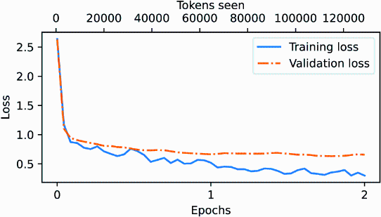
Figure 7.17 The training and validation loss trends over two epochs. The solid line represents the training loss, showing a sharp decrease before stabilizing, while the dotted line represents the validation loss, which follows a similar pattern.
While the loss plot in figure 7.17 indicates that the model is training effectively, the most crucial aspect is its performance in terms of response quality and correctness. So, next, let’s extract the responses and store them in a format that allows us to evaluate and quantify the response quality.
7.7 Extracting and saving responses
Having fine-tuned the LLM on the training portion of the instruction dataset, we are now ready to evaluate its performance on the held-out test set. First, we extract the model-generated responses for each input in the test dataset and collect them for manual analysis, and then we evaluate the LLM to quantify the quality of the responses, as highlighted in figure 7.18.
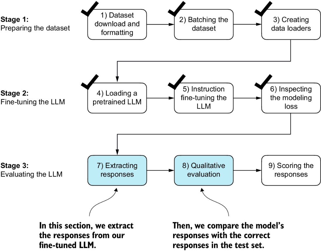
Figure 7.18 The three-stage process for instruction fine-tuning the LLM. In the first two steps of stage 3, we extract and collect the model responses on the held-out test dataset for further analysis and then evaluate the model to quantify the performance of the instruction-fine-tuned LLM.
To complete the response instruction step, we use the generate function. We then print the model responses alongside the expected test set answers for the first three test set entries, presenting them side by side for comparison:
torch.manual_seed(123)

for entry in test_data[:3]:      #1
    input_text = format_input(entry)
    token_ids = generate(               #2
        model=model,
        idx=text_to_token_ids(input_text, tokenizer).to(device),
        max_new_tokens=256,
        context_size=BASE_CONFIG["context_length"],
        eos_id=50256
    )
    generated_text = token_ids_to_text(token_ids, tokenizer)

    response_text = (
        generated_text[len(input_text):]
        .replace("### Response:", "")
        .strip()
    )
    print(input_text)
    print(f"\nCorrect response:\\n>> {entry['output']}")
    print(f"\nModel response:\\n>> {response_text.strip()}")
    print("-------------------------------------")
As mentioned earlier, the generate function returns the combined input and output text, so we use slicing and the .replace() method on the generated_text contents to extract the model’s response. The instructions, followed by the given test set response and model response, are shown next.
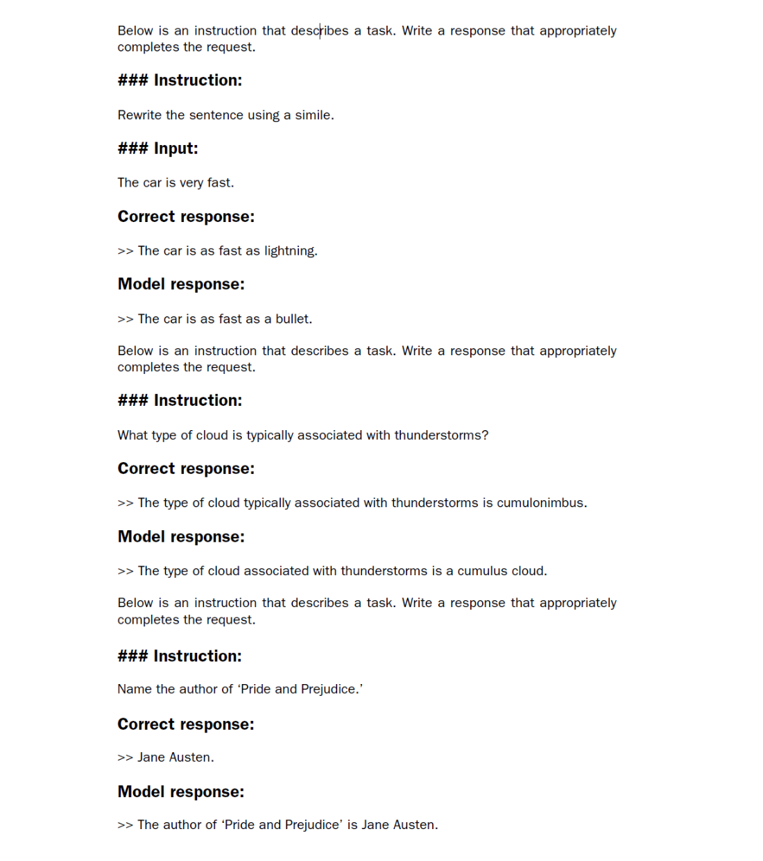
As we can see based on the test set instructions, given responses, and the model’s responses, the model performs relatively well. The answers to the first and last instructions are clearly correct, while the second answer is close but not entirely accurate. The model answers with “cumulus cloud” instead of “cumulonimbus,” although it’s worth noting that cumulus clouds can develop into cumulonimbus clouds, which are capable of producing thunderstorms.
Most importantly, model evaluation is not as straightforward as it is for completion fine-tuning, where we simply calculate the percentage of correct spam/non-spam class labels to obtain the classification’s accuracy. In practice, instruction-fine-tuned LLMs such as chatbots are evaluated via multiple approaches:
- Short-answer and multiple-choice benchmarks, such as Measuring Massive Multitask Language Understanding (MMLU; https://arxiv.org/abs/2009.03300), which test the general knowledge of a model.
- Human preference comparison to other LLMs, such as LMSYS chatbot arena (https://arena.lmsys.org).
- Automated conversational benchmarks, where another LLM like GPT-4 is used to evaluate the responses, such as AlpacaEval (https://tatsu-lab.github.io/alpaca_eval/).
In practice, it can be useful to consider all three types of evaluation methods: multiple-choice question answering, human evaluation, and automated metrics that measure conversational performance. However, since we are primarily interested in assessing conversational performance rather than just the ability to answer multiple-choice questions, human evaluation and automated metrics may be more relevant.
Human evaluation, while providing valuable insights, can be relatively laborious and time-consuming, especially when dealing with a large number of responses. For instance, reading and assigning ratings to all 1,100 responses would require a significant amount of effort.
So, considering the scale of the task at hand, we will implement an approach similar to automated conversational benchmarks, which involves evaluating the responses automatically using another LLM. This method will allow us to efficiently assess the quality of the generated responses without the need for extensive human involvement, thereby saving time and resources while still obtaining meaningful performance indicators.
Let’s employ an approach inspired by AlpacaEval, using another LLM to evaluate our fine-tuned model’s responses. However, instead of relying on a publicly available benchmark dataset, we use our own custom test set. This customization allows for a more targeted and relevant assessment of the model’s performance within the context of our intended use cases, represented in our instruction dataset.
To prepare the responses for this evaluation process, we append the generated model responses to the test_set dictionary and save the updated data as an "instruction-data-with-response.json" file for record keeping. Additionally, by saving this file, we can easily load and analyze the responses in separate Python sessions later on if needed.
The following code listing uses the generate method in the same manner as before; however, we now iterate over the entire test_set. Also, instead of printing the model responses, we add them to the test_set dictionary.
Listing 7.9 Generating test set responses
from tqdm import tqdm

for i, entry in tqdm(enumerate(test_data), total=len(test_data)):
    input_text = format_input(entry)

    token_ids = generate(
        model=model,
        idx=text_to_token_ids(input_text, tokenizer).to(device),
        max_new_tokens=256,
        context_size=BASE_CONFIG["context_length"],
        eos_id=50256
    )
    generated_text = token_ids_to_text(token_ids, tokenizer)

    response_text = (
        generated_text[len(input_text):]
        .replace("### Response:", "")
        .strip()
    )
    test_data[i]["model_response"] = response_text

with open("instruction-data-with-response.json", "w") as file:
    json.dump(test_data, file, indent=4)         #1
Processing the dataset takes about 1 minute on an A100 GPU and 6 minutes on an M3 MacBook Air:
100%|██████████| 110/110 [01:05<00:00, 1.68it/s]
Let’s verify that the responses have been correctly added to the test_set dictionary by examining one of the entries:
print(test_data[0])
The output shows that the model_response has been added correctly:
{'instruction': 'Rewrite the sentence using a simile.',
 'input': 'The car is very fast.',
 'output': 'The car is as fast as lightning.',
 'model_response': 'The car is as fast as a bullet.'}
Finally, we save the model as gpt2-medium355M-sft.pth file to be able to reuse it in future projects:
import re

file_name = f"{re.sub(r'[ ()]', '', CHOOSE_MODEL) }-sft.pth"      #1
torch.save(model.state_dict(), file_name)
print(f"Model saved as {file_name}")
The saved model can then be loaded via model.load_state_dict(torch.load("gpt2 -medium355M-sft.pth")).
7.8 Evaluating the fine-tuned LLM
Previously, we judged the performance of an instruction-fine-tuned model by looking at its responses on three examples of the test set. While this gives us a rough idea of how well the model performs, this method does not scale well to larger amounts of responses. So, we implement a method to automate the response evaluation of the fine-tuned LLM using another, larger LLM, as highlighted in figure 7.19.
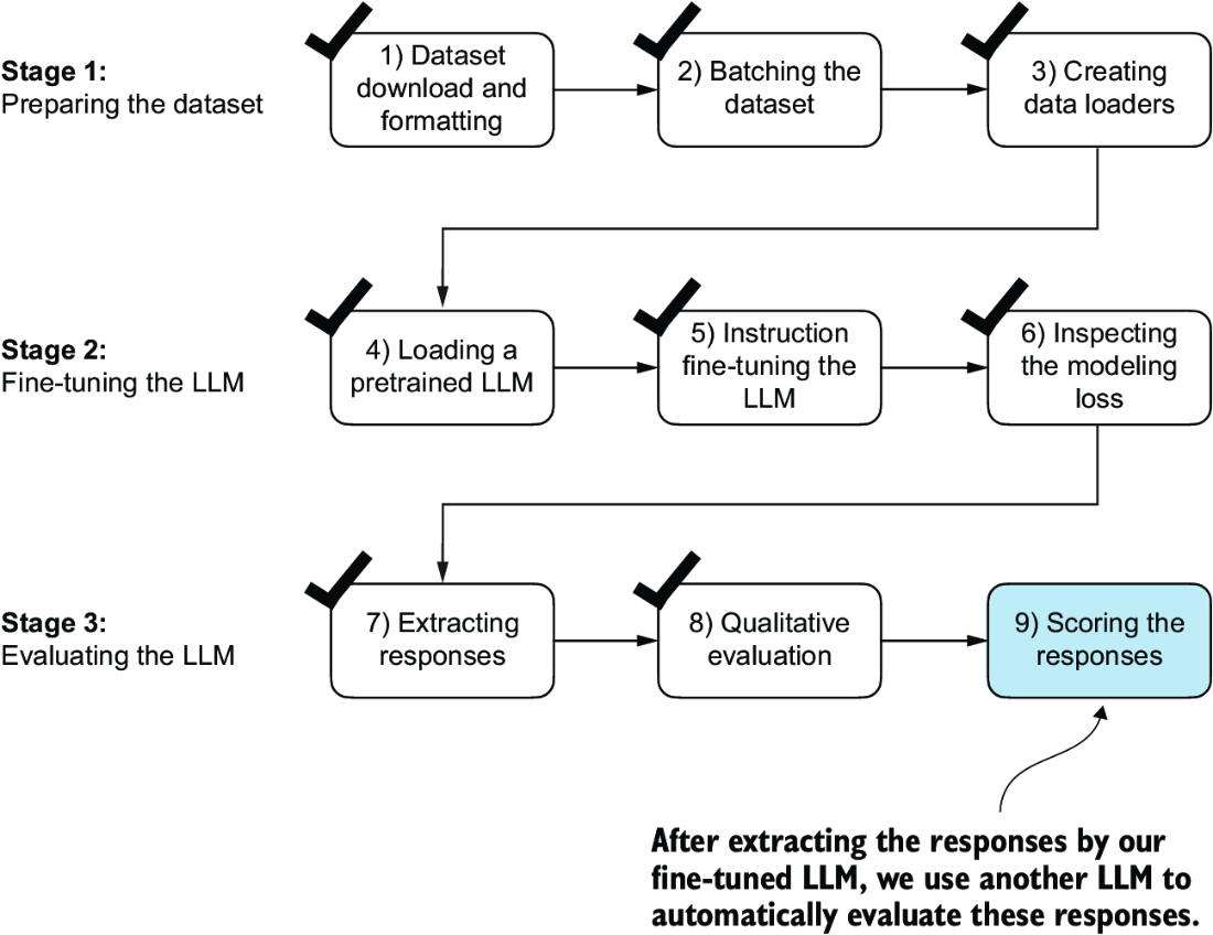
Figure 7.19 The three-stage process for instruction fine-tuning the LLM. In this last step of the instruction-fine-tuning pipeline, we implement a method to quantify the performance of the fine-tuned model by scoring the responses it generated for the test.
To evaluate test set responses in an automated fashion, we utilize an existing instruction-fine-tuned 8-billion-parameter Llama 3 model developed by Meta AI. This model can be run locally using the open source Ollama application (https://ollama.com).
NOTE Ollama is an efficient application for running LLMs on a laptop. It serves as a wrapper around the open source llama.cpp library (https://github.com/ggerganov/llama.cpp), which implements LLMs in pure C/C++ to maximize efficiency. However, Ollama is only a tool for generating text using LLMs (inference) and does not support training or fine-tuning LLMs.
To execute the following code, install Ollama by visiting https://ollama.comand follow the provided instructions for your operating system:
- For macOS and Windows users—Open the downloaded Ollama application. If prompted to install command-line usage, select Yes.
- For Linux users—Use the installation command available on the Ollama website.
Before implementing the model evaluation code, let’s first download the Llama 3 model and verify that Ollama is functioning correctly by using it from the command-line terminal. To use Ollama from the command line, you must either start the Ollama application or run ollama serve in a separate terminal, as shown in figure 7.20.
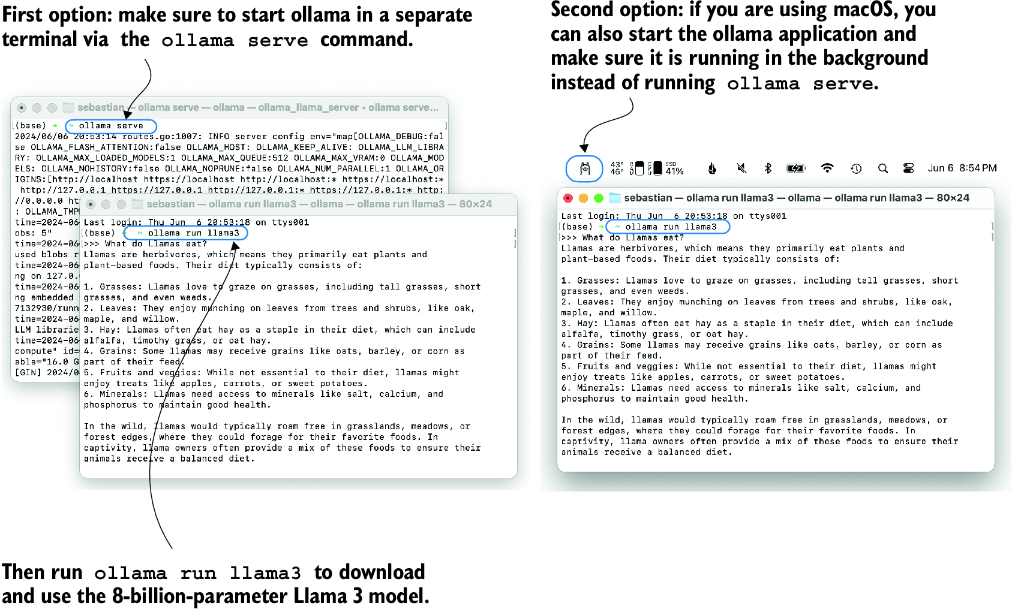
Figure 7.20 Two options for running Ollama. The left panel illustrates starting Ollama using ollama serve. The right panel shows a second option in macOS, running the Ollama application in the background instead of using the ollama serve command to start the application.
With the Ollama application or ollama serve running in a different terminal, execute the following command on the command line (not in a Python session) to try out the 8-billion-parameter Llama 3 model:
ollama run llama3
The first time you execute this command, this model, which takes up 4.7 GB of storage space, will be automatically downloaded. The output looks like the following:
pulling manifest
pulling 6a0746a1ec1a... 100% |████████████████| 4.7 GB
pulling 4fa551d4f938... 100% |████████████████|  12 KB
pulling 8ab4849b038c... 100% |████████████████|  254 B
pulling 577073ffcc6c... 100% |████████████████|  110 B
pulling 3f8eb4da87fa... 100% |████████████████|  485 B
verifying sha256 digest
writing manifest
removing any unused layers
success
Once the model download is complete, we are presented with a command-line interface that allows us to interact with the model. For example, try asking the model, “What do llamas eat?”
>>> What do llamas eat?
Llamas are ruminant animals, which means they have a four-chambered
stomach and eat plants that are high in fiber. In the wild,
llamas typically feed on:

1. Grasses: They love to graze on various types of grasses, including tall
grasses, wheat, oats, and barley.
Note that the response you see might differ since Ollama is not deterministic as of this writing.
You can end this ollama run llama3 session using the input /bye. However, make sure to keep the ollama serve command or the Ollama application running for the remainder of this chapter.
The following code verifies that the Ollama session is running properly before we use Ollama to evaluate the test set responses:
import psutil

def check_if_running(process_name):
    running = False
    for proc in psutil.process_iter(["name"]):
        if process_name in proc.info["name"]:
            running = True
            break
    return running

ollama_running = check_if_running("ollama")

if not ollama_running:
    raise RuntimeError(
        "Ollama not running. Launch ollama before proceeding."
)
print("Ollama running:", check_if_running("ollama"))
Ensure that the output from executing the previous code displays Ollama running: True. If it shows False, verify that the ollama serve command or the Ollama application is actively running.
An alternative to the ollama run command for interacting with the model is through its REST API using Python. The query_model function shown in the following listing demonstrates how to use the API.
Listing 7.10 Querying a local Ollama model
import urllib.request

def query_model(
    prompt,
    model="llama3",
    url="http://localhost:11434/api/chat"
):
    data = {             #1
        "model": model,
        "messages": [
            {"role": "user", "content": prompt}
        ],
        "options": {         #2
            "seed": 123,
            "temperature": 0,
            "num_ctx": 2048
        }
    }


    payload = json.dumps(data).encode("utf-8")    #3
    request = urllib.request.Request(                       #4
        url,                                                #4
        data=payload,                                       #4
        method="POST"                                       #4
    ) #4

    request.add_header("Content-Type", "application/json")   #4

    response_data = ""
    with urllib.request.urlopen(request) as response:   #5
        while True:
            line = response.readline().decode("utf-8")
            if not line:
                break
            response_json = json.loads(line)
            response_data += response_json["message"]["content"]

    return response_data
Before running the subsequent code cells in this notebook, ensure that Ollama is still running. The previous code cells should print "Ollama running: True" to confirm that the model is active and ready to receive requests.
The following is an example of how to use the query_model function we just implemented:
model = "llama3"
result = query_model("What do Llamas eat?", model)
print(result)
The resulting response is as follows:
Llamas are ruminant animals, which means they have a four-chambered
stomach that allows them to digest plant-based foods. Their diet
typically consists of:

1. Grasses: Llamas love to graze on grasses, including tall grasses,
short grasses, and even weeds.
...
Using the query_model function defined earlier, we can evaluate the responses generated by our fine-tuned model that prompts the Llama 3 model to rate our fine-tuned model’s responses on a scale from 0 to 100 based on the given test set response as reference.
First, we apply this approach to the first three examples from the test set that we previously examined:
for entry in test_data[:3]:
    prompt = (
        f"Given the input `{format_input(entry)}` "
        f"and correct output `{entry['output']}`, "
        f"score the model response `{entry['model_response']}`"
        f" on a scale from 0 to 100, where 100 is the best score. "
    )
    print("\nDataset response:")
    print(">>", entry['output'])
    print("\nModel response:")
    print(">>", entry["model_response"])
    print("\nScore:")
    print(">>", query_model(prompt))
    print("\n-------------------------")
This code prints outputs similar to the following (as of this writing, Ollama is not fully deterministic, so the generated texts may vary):
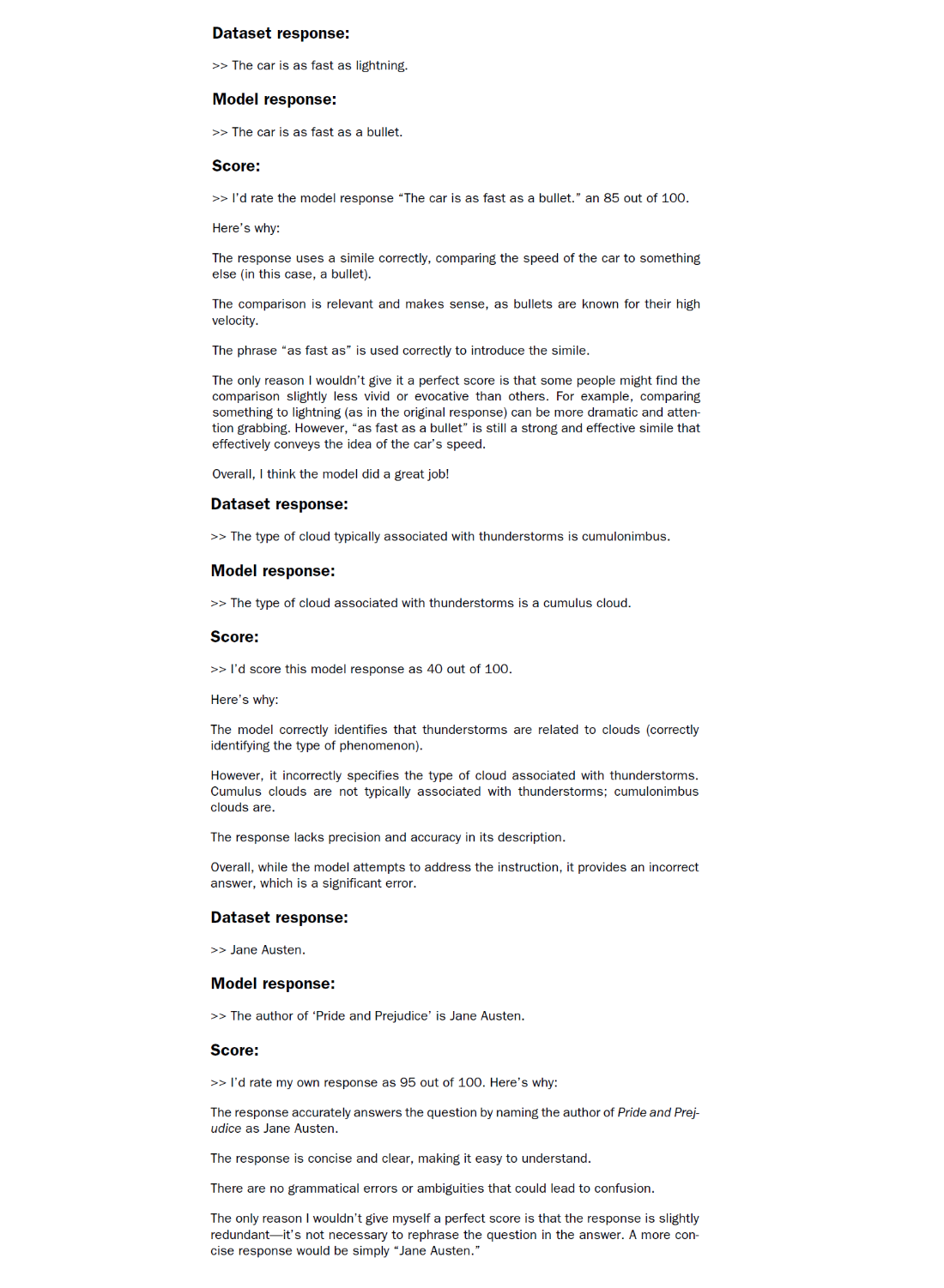
The generated responses show that the Llama 3 model provides reasonable evaluations and is capable of assigning partial points when a model’s answer is not entirely correct. For instance, if we consider the evaluation of the “cumulus cloud” answer, the model acknowledges the partial correctness of the response.
The previous prompt returns highly detailed evaluations in addition to the score. We can modify the prompt to just generate integer scores ranging from 0 to 100, where 100 represents the best possible score. This modification allows us to calculate an average score for our model, which serves as a more concise and quantitative assessment of its performance. The generate_model_scores function shown in the following listing uses a modified prompt telling the model to "Respond with the integer number only."
Listing 7.11 Evaluating the instruction fine-tuning LLM
def generate_model_scores(json_data, json_key, model="llama3"):
    scores = []
    for entry in tqdm(json_data, desc="Scoring entries"):
        prompt = (
            f"Given the input `{format_input(entry)}` "
            f"and correct output `{entry['output']}`, "
            f"score the model response `{entry[json_key]}`"
            f" on a scale from 0 to 100, where 100 is the best score. "
            f"Respond with the integer number only."   #1
        )
        score = query_model(prompt, model)
        try:
            scores.append(int(score))
        except ValueError:
            print(f"Could not convert score: {score}")
            continue

    return scores
Let’s now apply the generate_model_scores function to the entire test_data set, which takes about 1 minute on a M3 Macbook Air:
scores = generate_model_scores(test_data, "model_response")
print(f"Number of scores: {len(scores)} of {len(test_data)}")
print(f"Average score: {sum(scores)/len(scores):.2f}\n")
The results are as follows:
Scoring entries: 100%|████████████████████████| 110/110
[01:10<00:00,  1.56it/s]
Number of scores: 110 of 110
Average score: 50.32
The evaluation output shows that our fine-tuned model achieves an average score above 50, which provides a useful benchmark for comparison against other models or for experimenting with different training configurations to improve the model’s performance.
It’s worth noting that Ollama is not entirely deterministic across operating systems at the time of this writing, which means that the scores you obtain might vary slightly from the previous scores. To obtain more robust results, you can repeat the evaluation multiple times and average the resulting scores.
To further improve our model’s performance, we can explore various strategies, such as
- Adjusting the hyperparameters during fine-tuning, such as the learning rate, batch size, or number of epochs
- Increasing the size of the training dataset or diversifying the examples to cover a broader range of topics and styles
- Experimenting with different prompts or instruction formats to guide the model’s responses more effectively
- Using a larger pretrained model, which may have greater capacity to capture complex patterns and generate more accurate responses
NOTE For reference, when using the methodology described herein, the Llama 3 8B base model, without any fine-tuning, achieves an average score of 58.51 on the test set. The Llama 3 8B instruct model, which has been fine-tuned on a general instruction-following dataset, achieves an impressive average score of 82.6.
7.9 Conclusions
This chapter marks the conclusion of our journey through the LLM development cycle. We have covered all the essential steps, including implementing an LLM architecture, pretraining an LLM, and fine-tuning it for specific tasks, as summarized in figure 7.21. Let’s discuss some ideas for what to look into next.

Figure 7.21 The three main stages of coding an LLM.
7.9.1 What’s next?
While we covered the most essential steps, there is an optional step that can be performed after instruction fine-tuning: preference fine-tuning. Preference fine-tuning is particularly useful for customizing a model to better align with specific user preferences. If you are interested in exploring this further, see the 04_preference-tuning-with-dpo folder in this book’s supplementary GitHub repository at https://mng.bz/dZwD.
In addition to the main content covered in this book, the GitHub repository also contains a large selection of bonus material that you may find valuable. To learn more about these additional resources, visit the Bonus Material section on the repository’s README page: https://mng.bz/r12g.
7.9.2 Staying up to date in a fast-moving field
The fields of AI and LLM research are evolving at a rapid (and, depending on who you ask, exciting) pace. One way to keep up with the latest advancements is to explore recent research papers on arXiv at https://arxiv.org/list/cs.LG/recent. Additionally, many researchers and practitioners are very active in sharing and discussing the latest developments on social media platforms like X (formerly Twitter) and Reddit. The subreddit r/LocalLLaMA, in particular, is a good resource for connecting with the community and staying informed about the latest tools and trends. I also regularly share insights and write about the latest in LLM research on my blog, available at https://magazine.sebastianraschka.com and https://sebastianraschka.com/blog/.
7.9.3 Final words
I hope you have enjoyed this journey of implementing an LLM from the ground up and coding the pretraining and fine-tuning functions from scratch. In my opinion, building an LLM from scratch is the most effective way to gain a deep understanding of how LLMs work. I hope that this hands-on approach has provided you with valuable insights and a solid foundation in LLM development.
While the primary purpose of this book is educational, you may be interested in utilizing different and more powerful LLMs for real-world applications. For this, I recommend exploring popular tools such as Axolotl (https://github.com/OpenAccess-AI-Collective/axolotl) or LitGPT (https://github.com/Lightning-AI/litgpt), which I am actively involved in developing.
Thank you for joining me on this learning journey, and I wish you all the best in your future endeavors in the exciting field of LLMs and AI!
Summary
- The instruction-fine-tuning process adapts a pretrained LLM to follow human instructions and generate desired responses.
- Preparing the dataset involves downloading an instruction-response dataset, formatting the entries, and splitting it into train, validation, and test sets.
- Training batches are constructed using a custom collate function that pads sequences, creates target token IDs, and masks padding tokens.
- We load a pretrained GPT-2 medium model with 355 million parameters to serve as the starting point for instruction fine-tuning.
- The pretrained model is fine-tuned on the instruction dataset using a training loop similar to pretraining.
- Evaluation involves extracting model responses on a test set and scoring them (for example, using another LLM).
- The Ollama application with an 8-billion-parameter Llama model can be used to automatically score the fine-tuned model’s responses on the test set, providing an average score to quantify performance.