appendix D Adding bells and whistles to the training loop
In this appendix, we enhance the training function for the pretraining and fine-tuning processes covered in chapters 5 to 7. In particular, it covers learning rate warmup, cosine decay, and gradient clipping. We then incorporate these techniques into the training function and pretrain an LLM.
To make the code self-contained, we reinitialize the model we trained in chapter 5:
import torch
from chapter04 import GPTModel

GPT_CONFIG_124M = {
    "vocab_size": 50257,          #1

    "context_length": 256,       #2
    "emb_dim": 768,           #3
    "n_heads": 12,            #4
    "n_layers": 12,           #5
    "drop_rate": 0.1,         #6
    "qkv_bias": False         #7
}
device = torch.device("cuda" if torch.cuda.is_available() else "cpu")
torch.manual_seed(123)
model = GPTModel(GPT_CONFIG_124M)
model.to(device)
model.eval()
After initializing the model, we need to initialize the data loaders. First, we load the “The Verdict” short story:
import os
import urllib.request

file_path = "the-verdict.txt"

url = (
    "https://raw.githubusercontent.com/rasbt/LLMs-from-scratch/"
    "main/ch02/01_main-chapter-code/the-verdict.txt"
)

if not os.path.exists(file_path):
    with urllib.request.urlopen(url) as response:
        text_data = response.read().decode('utf-8')
    with open(file_path, "w", encoding="utf-8") as file:
        file.write(text_data)
else:
    with open(file_path, "r", encoding="utf-8") as file:
        text_data = file.read()
Next, we load the text_data into the data loaders:
from previous_chapters import create_dataloader_v1

train_ratio = 0.90
split_idx = int(train_ratio * len(text_data))
torch.manual_seed(123)
train_loader = create_dataloader_v1(
    text_data[:split_idx],
    batch_size=2,
    max_length=GPT_CONFIG_124M["context_length"],
    stride=GPT_CONFIG_124M["context_length"],
    drop_last=True,
    shuffle=True,
    num_workers=0
)
val_loader = create_dataloader_v1(
    text_data[split_idx:],
    batch_size=2,
    max_length=GPT_CONFIG_124M["context_length"],
    stride=GPT_CONFIG_124M["context_length"],
    drop_last=False,
    shuffle=False,
    num_workers=0
)
D.1 Learning rate warmup
Implementing a learning rate warmup can stabilize the training of complex models such as LLMs. This process involves gradually increasing the learning rate from a very low initial value (initial_lr) to a maximum value specified by the user (peak_lr). Starting the training with smaller weight updates decreases the risk of the model encountering large, destabilizing updates during its training phase.
Suppose we plan to train an LLM for 15 epochs, starting with an initial learning rate of 0.0001 and increasing it to a maximum learning rate of 0.01:
n_epochs = 15
initial_lr = 0.0001
peak_lr = 0.01
warmup_steps = 20
The number of warmup steps is usually set between 0.1% and 20% of the total number of steps, which we can calculate as follows:
total_steps = len(train_loader) * n_epochs
warmup_steps = int(0.2 * total_steps)       #1
print(warmup_steps)
This prints 27, meaning that we have 20 warmup steps to increase the initial learning rate from 0.0001 to 0.01 in the first 27 training steps.
Next, we implement a simple training loop template to illustrate this warmup process:
optimizer = torch.optim.AdamW(model.parameters(), weight_decay=0.1)
lr_increment = (peak_lr - initial_lr) / warmup_steps    #1

global_step = -1
track_lrs = []

for epoch in range(n_epochs):    #2
    for input_batch, target_batch in train_loader:
        optimizer.zero_grad()
        global_step += 1

        if global_step < warmup_steps:             #3
            lr = initial_lr + global_step * lr_increment
        else:
            lr = peak_lr

        for param_group in optimizer.param_groups:    #4
            param_group["lr"] = lr
        track_lrs.append(optimizer.param_groups[0]["lr"])   #5
After running the preceding code, we visualize how the learning rate was changed by the training loop to verify that the learning rate warmup works as intended:
import matplotlib.pyplot as plt

plt.ylabel("Learning rate")
plt.xlabel("Step")
total_training_steps = len(train_loader) * n_epochs
plt.plot(range(total_training_steps), track_lrs);
plt.show()
The resulting plot shows that the learning rate starts with a low value and increases for 20 steps until it reaches the maximum value after 20 steps (figure D.1).
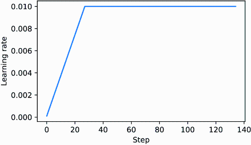
Figure D.1 The learning rate warmup increases the learning rate for the first 20 training steps. After 20 steps, the learning rate reaches the peak of 0.01 and remains constant for the rest of the training.
Next, we will modify the learning rate further so that it decreases after reaching the maximum learning rate, which further helps improve the model training.
D.2 Cosine decay
Another widely adopted technique for training complex deep neural networks and LLMs is cosine decay. This method modulates the learning rate throughout the training epochs, making it follow a cosine curve after the warmup stage.
In its popular variant, cosine decay reduces (or decays) the learning rate to nearly zero, mimicking the trajectory of a half-cosine cycle. The gradual learning decrease in cosine decay aims to decelerate the pace at which the model updates its weights. This is particularly important because it helps minimize the risk of overshooting the loss minima during the training process, which is essential for ensuring the stability of the training during its later phases.
We can modify the training loop template by adding cosine decay:
import math

min_lr = 0.1 * initial_lr
track_lrs = []
lr_increment = (peak_lr - initial_lr) / warmup_steps
global_step = -1

for epoch in range(n_epochs):
    for input_batch, target_batch in train_loader:
        optimizer.zero_grad()
        global_step += 1

        if global_step < warmup_steps:                     #1
            lr = initial_lr + global_step * lr_increment
        else:                                                #2
            progress = ((global_step - warmup_steps) /
                        (total_training_steps - warmup_steps))
            lr = min_lr + (peak_lr - min_lr) * 0.5 * (
                1 + math.cos(math.pi * progress)
            )

        for param_group in optimizer.param_groups:
            param_group["lr"] = lr
        track_lrs.append(optimizer.param_groups[0]["lr"])
Again, to verify that the learning rate has changed as intended, we plot the learning rate:
plt.ylabel("Learning rate")
plt.xlabel("Step")
plt.plot(range(total_training_steps), track_lrs)
plt.show()
The resulting learning rate plot shows that the learning rate starts with a linear warmup phase, which increases for 20 steps until it reaches the maximum value after 20 steps. After the 20 steps of linear warmup, cosine decay kicks in, reducing the learning rate gradually until it reaches its minimum (figure D.2).
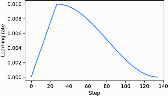
Figure D.2 The first 20 steps of linear learning rate warmup are followed by a cosine decay, which reduces the learning rate in a half-cosine cycle until it reaches its minimum point at the end of training.
D.3 Gradient clipping
Gradient clipping is another important technique for enhancing stability during LLM training. This method involves setting a threshold above which gradients are downscaled to a predetermined maximum magnitude. This process ensures that the updates to the model’s parameters during backpropagation stay within a manageable range.
For example, applying the max_norm=1.0 setting within PyTorch’s clip_grad_ norm_ function ensures that the norm of the gradients does not surpass 1.0. Here, the term “norm” signifies the measure of the gradient vector’s length, or magnitude, within the model’s parameter space, specifically referring to the L2 norm, also known as the Euclidean norm.
In mathematical terms, for a vector v composed of components v = [v1, v2, ..., vn], the L2 norm is
This calculation method is also applied to matrices. For instance, consider a gradient matrix given by
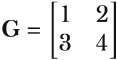
If we want to clip these gradients to a max_norm of 1, we first compute the L2 norm of these gradients, which is
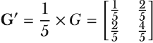
Given that |G|2 = 5 exceeds our max_norm of 1, we scale down the gradients to ensure their norm equals exactly 1. This is achieved through a scaling factor, calculated as max_norm/|G|2 = 1/5. Consequently, the adjusted gradient matrix G' becomes
To illustrate this gradient clipping process, we begin by initializing a new model and calculating the loss for a training batch, similar to the procedure in a standard training loop:
from chapter05 import calc_loss_batch

torch.manual_seed(123)
model = GPTModel(GPT_CONFIG_124M)
model.to(device)
loss = calc_loss_batch(input_batch, target_batch, model, device)
loss.backward()
Upon calling the .backward() method, PyTorch calculates the loss gradients and stores them in a .grad attribute for each model weight (parameter) tensor.
To clarify the point, we can define the following find_highest_gradient utility function to identify the highest gradient value by scanning all the .grad attributes of the model’s weight tensors after calling .backward():
def find_highest_gradient(model):
    max_grad = None
    for param in model.parameters():
        if param.grad is not None:
            grad_values = param.grad.data.flatten()
            max_grad_param = grad_values.max()
            if max_grad is None or max_grad_param > max_grad:
                max_grad = max_grad_param
    return max_grad
print(find_highest_gradient(model))
The largest gradient value identified by the preceding code is
tensor(0.0411)
Let’s now apply gradient clipping and see how this affects the largest gradient value:
torch.nn.utils.clip_grad_norm_(model.parameters(), max_norm=1.0)
print(find_highest_gradient(model))
The largest gradient value after applying the gradient clipping with the max norm of 1 is substantially smaller than before:
tensor(0.0185)
D.4 The modified training function
Finally, we improve the train_model_simple training function (see chapter 5) by adding the three concepts introduced herein: linear warmup, cosine decay, and gradient clipping. Together, these methods help stabilize LLM training.
The code, with the changes compared to the train_model_simple annotated, is as follows:
from chapter05 import evaluate_model, generate_and_print_sample


def train_model(model, train_loader, val_loader, optimizer, device,
                n_epochs, eval_freq, eval_iter, start_context, tokenizer,
                warmup_steps, initial_lr=3e-05, min_lr=1e-6):

    train_losses, val_losses, track_tokens_seen, track_lrs = [], [], [], []
    tokens_seen, global_step = 0, -1

    peak_lr = optimizer.param_groups[0]["lr"]   #1
    total_training_steps = len(train_loader) * n_epochs     #2
    lr_increment = (peak_lr - initial_lr) / warmup_steps    #3

    for epoch in range(n_epochs):
        model.train()
        for input_batch, target_batch in train_loader:
            optimizer.zero_grad()
            global_step += 1

            if global_step < warmup_steps:   #4
                lr = initial_lr + global_step * lr_increment
            else:
                progress = ((global_step - warmup_steps) /
                            (total_training_steps - warmup_steps))
                lr = min_lr + (peak_lr - min_lr) * 0.5 * (
                    1 + math.cos(math.pi * progress))

            for param_group in optimizer.param_groups:   #5
                param_group["lr"] = lr
            track_lrs.append(lr)
            loss = calc_loss_batch(input_batch, target_batch, model, device)
            loss.backward()

            if global_step > warmup_steps:         #6
                torch.nn.utils.clip_grad_norm_(
                    model.parameters(), max_norm=1.0
                )
 #7
            optimizer.step()
            tokens_seen += input_batch.numel()

            if global_step % eval_freq == 0:
                train_loss, val_loss = evaluate_model(
                    model, train_loader, val_loader,
                    device, eval_iter
                )
                train_losses.append(train_loss)
                val_losses.append(val_loss)
                track_tokens_seen.append(tokens_seen)
                print(f"Ep {epoch+1} (Iter {global_step:06d}): "
                      f"Train loss {train_loss:.3f}, "
                      f"Val loss {val_loss:.3f}"
                )


        generate_and_print_sample(
            model, tokenizer, device, start_context
        )

    return train_losses, val_losses, track_tokens_seen, track_lrs
After defining the train_model function, we can use it in a similar fashion to train the model compared to the train_model_simple method we used for pretraining:
import tiktoken

torch.manual_seed(123)
model = GPTModel(GPT_CONFIG_124M)
model.to(device)
peak_lr = 5e-4
optimizer = torch.optim.AdamW(model.parameters(), weight_decay=0.1)
tokenizer = tiktoken.get_encoding("gpt2")

n_epochs = 15
train_losses, val_losses, tokens_seen, lrs = train_model(
    model, train_loader, val_loader, optimizer, device, n_epochs=n_epochs,
    eval_freq=5, eval_iter=1, start_context="Every effort moves you",
    tokenizer=tokenizer, warmup_steps=warmup_steps,
    initial_lr=1e-5, min_lr=1e-5
)
The training will take about 5 minutes to complete on a MacBook Air or similar laptop and prints the following outputs:
Ep 1 (Iter 000000): Train loss 10.934, Val loss 10.939
Ep 1 (Iter 000005): Train loss 9.151, Val loss 9.461
Every effort moves you,,,,,,,,,,,,,,,,,,,,,,,,,,,,,,,,,,,,,,,,,,,,,,,,,,
Ep 2 (Iter 000010): Train loss 7.949, Val loss 8.184
Ep 2 (Iter 000015): Train loss 6.362, Val loss 6.876
Every effort moves you,,,,,,,,,,,,,,,,,,, the,,,,,,,,, the,,,,,,,,,,,
the,,,,,,,,
...
Ep 15 (Iter 000130): Train loss 0.041, Val loss 6.915
Every effort moves you?"  "Yes--quite insensible to the irony. She wanted him vindicated--and by me!"  He laughed again, and threw back his head to look up at the sketch of the donkey. "There were days when I
Like pretraining, the model begins to overfit after a few epochs since it is a very small dataset, and we iterate over it multiple times. Nonetheless, we can see that the function is working since it minimizes the training set loss.
Readers are encouraged to train the model on a larger text dataset and compare the results obtained with this more sophisticated training function to the results that can be obtained with the train_model_simple function.