appendix E Parameter-efficient fine-tuning with LoRA
Low-rank adaptation (LoRA) is one of the most widely used techniques for parameter-efficient fine-tuning. The following discussion is based on the spam classification fine-tuning example given in chapter 6. However, LoRA fine-tuning is also applicable to the supervised instruction fine-tuning discussed in chapter 7.
E.1 Introduction to LoRA
LoRA is a technique that adapts a pretrained model to better suit a specific, often smaller dataset by adjusting only a small subset of the model’s weight parameters. The “low-rank” aspect refers to the mathematical concept of limiting model adjustments to a smaller dimensional subspace of the total weight parameter space. This effectively captures the most influential directions of the weight parameter changes during training. The LoRA method is useful and popular because it enables efficient fine-tuning of large models on task-specific data, significantly cutting down on the computational costs and resources usually required for fine-tuning.
Suppose a large weight matrix W is associated with a specific layer. LoRA can be applied to all linear layers in an LLM. However, we focus on a single layer for illustration purposes.
When training deep neural networks, during backpropagation, we learn a DW matrix, which contains information on how much we want to update the original weight parameters to minimize the loss function during training. Hereafter, I use the term “weight” as shorthand for the model’s weight parameters.
In regular training and fine-tuning, the weight update is defined as follows:
The LoRA method, proposed by Hu et al. (https://arxiv.org/abs/2106.09685), offers a more efficient alternative to computing the weight updates DW by learning an approximation of it:
where A and B are two matrices much smaller than W, and AB represents the matrix multiplication product between A and B.
Using LoRA, we can then reformulate the weight update we defined earlier:
Figure E.1 illustrates the weight update formulas for full fine-tuning and LoRA side by side.
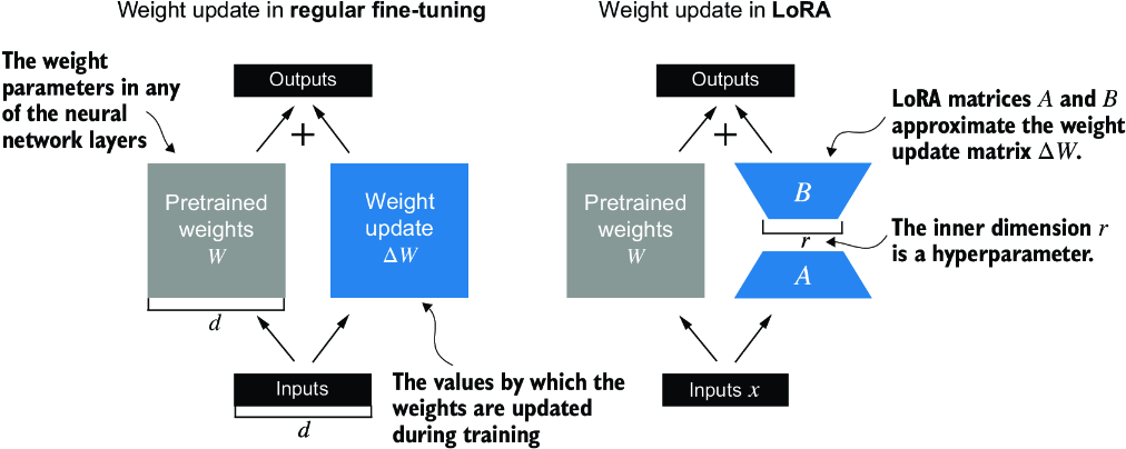
Figure E.1 A comparison between weight update methods: regular fine-tuning and LoRA. Regular fine-tuning involves updating the pretrained weight matrix W directly with DW (left). LoRA uses two smaller matrices, A and B, to approximate DW, where the product AB is added to W, and r denotes the inner dimension, a tunable hyperparameter (right).
If you paid close attention, you might have noticed that the visual representations of full fine-tuning and LoRA in figure E.1 differ slightly from the earlier presented formulas. This variation is attributed to the distributive law of matrix multiplication, which allows us to separate the original and updated weights rather than combine them. For example, in the case of regular fine-tuning with x as the input data, we can express the computation as
Similarly, we can write the following for LoRA:
Besides reducing the number of weights to update during training, the ability to keep the LoRA weight matrices separate from the original model weights makes LoRA even more useful in practice. Practically, this allows for the pretrained model weights to remain unchanged, with the LoRA matrices being applied dynamically after training when using the model.
Keeping the LoRA weights separate is very useful in practice because it enables model customization without needing to store multiple complete versions of an LLM. This reduces storage requirements and improves scalability, as only the smaller LoRA matrices need to be adjusted and saved when we customize LLMs for each specific customer or application.
Next, let’s see how LoRA can be used to fine-tune an LLM for spam classification, similar to the fine-tuning example in chapter 6.
E.2 Preparing the dataset
Before applying LoRA to the spam classification example, we must load the dataset and pretrained model we will work with. The code here repeats the data preparation from chapter 6. (Instead of repeating the code, we could open and run the chapter 6 notebook and insert the LoRA code from section E.4 there.)
First, we download the dataset and save it as CSV files.
Listing E.1 Downloading and preparing the dataset
from pathlib import Path
import pandas as pd
from ch06 import (
    download_and_unzip_spam_data,
    create_balanced_dataset,
    random_split
)

url = \
"https://archive.ics.uci.edu/static/public/228/sms+spam+collection.zip"
zip_path = "sms_spam_collection.zip"
extracted_path = "sms_spam_collection"
data_file_path = Path(extracted_path) / "SMSSpamCollection.tsv"

download_and_unzip_spam_data(url, zip_path, extracted_path, data_file_path)

df = pd.read_csv(
    data_file_path, sep="\t", header=None, names=["Label", "Text"]
)
balanced_df = create_balanced_dataset(df)
balanced_df["Label"] = balanced_df["Label"].map({"ham": 0, "spam": 1})

train_df, validation_df, test_df = random_split(balanced_df, 0.7, 0.1)
train_df.to_csv("train.csv", index=None)
validation_df.to_csv("validation.csv", index=None)
test_df.to_csv("test.csv", index=None)
Next, we create the SpamDataset instances.
Listing E.2 Instantiating PyTorch datasets
import torch
from torch.utils.data import Dataset
import tiktoken
from chapter06 import SpamDataset

tokenizer = tiktoken.get_encoding("gpt2")
train_dataset = SpamDataset("train.csv", max_length=None,
    tokenizer=tokenizer
)
val_dataset = SpamDataset("validation.csv",
    max_length=train_dataset.max_length, tokenizer=tokenizer
)
test_dataset = SpamDataset(
    "test.csv", max_length=train_dataset.max_length, tokenizer=tokenizer
)
After creating the PyTorch dataset objects, we instantiate the data loaders.
Listing E.3 Creating PyTorch data loaders
from torch.utils.data import DataLoader

num_workers = 0
batch_size = 8

torch.manual_seed(123)

train_loader = DataLoader(
    dataset=train_dataset,
    batch_size=batch_size,
    shuffle=True,
    num_workers=num_workers,
    drop_last=True,
)

val_loader = DataLoader(
    dataset=val_dataset,
    batch_size=batch_size,
    num_workers=num_workers,
    drop_last=False,
)

test_loader = DataLoader(
    dataset=test_dataset,
    batch_size=batch_size,
    num_workers=num_workers,
    drop_last=False,
)
As a verification step, we iterate through the data loaders and check that the batches contain eight training examples each, where each training example consists of 120 tokens:
print("Train loader:")
for input_batch, target_batch in train_loader:
    pass

print("Input batch dimensions:", input_batch.shape)
print("Label batch dimensions", target_batch.shape)
The output is
Train loader:
Input batch dimensions: torch.Size([8, 120])
Label batch dimensions torch.Size([8])
Lastly, we print the total number of batches in each dataset:
print(f"{len(train_loader)} training batches")
print(f"{len(val_loader)} validation batches")
print(f"{len(test_loader)} test batches")
In this case, we have the following number of batches per dataset:
130 training batches
19 validation batches
38 test batches
E.3 Initializing the model
We repeat the code from chapter 6 to load and prepare the pretrained GPT model. We begin by downloading the model weights and loading them into the GPTModel class.
Listing E.4 Loading a pretrained GPT model
from gpt_download import download_and_load_gpt2
from chapter04 import GPTModel
from chapter05 import load_weights_into_gpt


CHOOSE_MODEL = "gpt2-small (124M)"
INPUT_PROMPT = "Every effort moves"

BASE_CONFIG = {
    "vocab_size": 50257,         #1
    "context_length": 1024,      #2
    "drop_rate": 0.0,            #3
    "qkv_bias": True             #4
}

model_configs = {
    "gpt2-small (124M)": {"emb_dim": 768, "n_layers": 12, "n_heads": 12},
    "gpt2-medium (355M)": {"emb_dim": 1024, "n_layers": 24, "n_heads": 16},
    "gpt2-large (774M)": {"emb_dim": 1280, "n_layers": 36, "n_heads": 20},
    "gpt2-xl (1558M)": {"emb_dim": 1600, "n_layers": 48, "n_heads": 25},
}

BASE_CONFIG.update(model_configs[CHOOSE_MODEL])

model_size = CHOOSE_MODEL.split(" ")[-1].lstrip("(").rstrip(")")
settings, params = download_and_load_gpt2(
    model_size=model_size, models_dir="gpt2"
)

model = GPTModel(BASE_CONFIG)
load_weights_into_gpt(model, params)
model.eval()
To ensure that the model was loaded corrected, let’s double-check that it generates coherent text:
from chapter04 import generate_text_simple
from chapter05 import text_to_token_ids, token_ids_to_text

text_1 = "Every effort moves you"

token_ids = generate_text_simple(
    model=model,
    idx=text_to_token_ids(text_1, tokenizer),
    max_new_tokens=15,
    context_size=BASE_CONFIG["context_length"]
)

print(token_ids_to_text(token_ids, tokenizer))
The following output shows that the model generates coherent text, which is an indicator that the model weights are loaded correctly:
Every effort moves you forward.
The first step is to understand the importance of your work
Next, we prepare the model for classification fine-tuning, similar to chapter 6, where we replace the output layer:
torch.manual_seed(123)
num_classes = 2
model.out_head = torch.nn.Linear(in_features=768, out_features=num_classes)
device = torch.device("cuda" if torch.cuda.is_available() else "cpu")
model.to(device)
Lastly, we calculate the initial classification accuracy of the not-fine-tuned model (we expect this to be around 50%, which means that the model is not able to distinguish between spam and nonspam messages yet reliably):
from chapter06 import calc_accuracy_loader

torch.manual_seed(123)
train_accuracy = calc_accuracy_loader(
    train_loader, model, device, num_batches=10
)
val_accuracy = calc_accuracy_loader(
    val_loader, model, device, num_batches=10
)
test_accuracy = calc_accuracy_loader(
    test_loader, model, device, num_batches=10
)


print(f"Training accuracy: {train_accuracy*100:.2f}%")
print(f"Validation accuracy: {val_accuracy*100:.2f}%")
print(f"Test accuracy: {test_accuracy*100:.2f}%")
The initial prediction accuracies are
Training accuracy: 46.25%
Validation accuracy: 45.00%
Test accuracy: 48.75%
E.4 Parameter-efficient fine-tuning with LoRA
Next, we modify and fine-tune the LLM using LoRA. We begin by initializing a LoRALayer that creates the matrices A and B, along with the alpha scaling factor and the rank (r) setting. This layer can accept an input and compute the corresponding output, as illustrated in figure E.2.
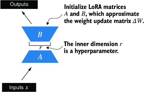
Figure E.2 The LoRA matrices A and B are applied to the layer inputs and are involved in computing the model outputs. The inner dimension r of these matrices serves as a setting that adjusts the number of trainable parameters by varying the sizes of A and B.
In code, this LoRA layer can be implemented as follows.
Listing E.5 Implementing a LoRA layer
import math

class LoRALayer(torch.nn.Module):
    def __init__(self, in_dim, out_dim, rank, alpha):
        super().__init__()
        self.A = torch.nn.Parameter(torch.empty(in_dim, rank))
        torch.nn.init.kaiming_uniform_(self.A, a=math.sqrt(5))    #1
        self.B = torch.nn.Parameter(torch.zeros(rank, out_dim))
        self.alpha = alpha

    def forward(self, x):
        x = self.alpha * (x @ self.A @ self.B)
        return x
The rank governs the inner dimension of matrices A and B. Essentially, this setting determines the number of extra parameters introduced by LoRA, which creates balance between the adaptability of the model and its efficiency via the number of parameters used.
The other important setting, alpha, functions as a scaling factor for the output from the low-rank adaptation. It primarily dictates the degree to which the output from the adapted layer can affect the original layer’s output. This can be seen as a way to regulate the effect of the low-rank adaptation on the layer’s output. The LoRALayer class we have implemented so far enables us to transform the inputs of a layer.
In LoRA, the typical goal is to substitute existing Linear layers, allowing weight updates to be applied directly to the pre-existing pretrained weights, as illustrated in figure E.3.
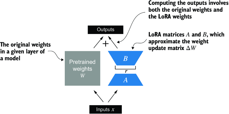
Figure E.3 The integration of LoRA into a model layer. The original pretrained weights (W) of a layer are combined with the outputs from LoRA matrices (A and B), which approximate the weight update matrix (DW). The final output is calculated by adding the output of the adapted layer (using LoRA weights) to the original output.
To integrate the original Linear layer weights, we now create a LinearWithLoRA layer. This layer utilizes the previously implemented LoRALayer and is designed to replace existing Linear layers within a neural network, such as the self-attention modules or feed-forward modules in the GPTModel.
Listing E.6 Replacing a LinearWithLora layer with Linear layers
class LinearWithLoRA(torch.nn.Module):
    def __init__(self, linear, rank, alpha):
        super().__init__()
        self.linear = linear
        self.lora = LoRALayer(
            linear.in_features, linear.out_features, rank, alpha
        )

    def forward(self, x):
        return self.linear(x) + self.lora(x)
This code combines a standard Linear layer with the LoRALayer. The forward method computes the output by adding the results from the original linear layer and the LoRA layer.
Since the weight matrix B (self.B in LoRALayer) is initialized with zero values, the product of matrices A and B results in a zero matrix. This ensures that the multiplication does not alter the original weights, as adding zero does not change them.
To apply LoRA to the earlier defined GPTModel, we introduce a replace_linear_ with_lora function. This function will swap all existing Linear layers in the model with the newly created LinearWithLoRA layers:
def replace_linear_with_lora(model, rank, alpha):
    for name, module in model.named_children():
        if isinstance(module, torch.nn.Linear):     #1
            setattr(model, name, LinearWithLoRA(module, rank, alpha))
        else:    #2
            replace_linear_with_lora(module, rank, alpha)
We have now implemented all the necessary code to replace the Linear layers in the GPTModel with the newly developed LinearWithLoRA layers for parameter-efficient fine-tuning. Next, we will apply the LinearWithLoRA upgrade to all Linear layers found in the multihead attention, feed-forward modules, and the output layer of the GPTModel, as shown in figure E.4.
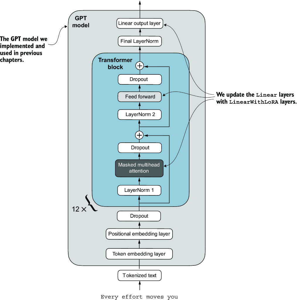
Figure E.4 The architecture of the GPT model. It highlights the parts of the model where Linear layers are upgraded to LinearWithLoRA layers for parameter-efficient fine-tuning.
Before we apply the LinearWithLoRA layer upgrades, we first freeze the original model parameters:
total_params = sum(p.numel() for p in model.parameters() if p.requires_grad)
print(f"Total trainable parameters before: {total_params:,}")

for param in model.parameters():
    param.requires_grad = False
total_params = sum(p.numel() for p in model.parameters() if p.requires_grad)
print(f"Total trainable parameters after: {total_params:,}")
Now, we can see that none of the 124 million model parameters are trainable:
Total trainable parameters before: 124,441,346
Total trainable parameters after: 0
Next, we use the replace_linear_with_lora to replace the Linear layers:
replace_linear_with_lora(model, rank=16, alpha=16)
total_params = sum(p.numel() for p in model.parameters() if p.requires_grad)
print(f"Total trainable LoRA parameters: {total_params:,}")
After adding the LoRA layers, the number of trainable parameters is as follows:
Total trainable LoRA parameters: 2,666,528
As we can see, we reduced the number of trainable parameters by almost 50× when using LoRA. A rank and alpha of 16 are good default choices, but it is also common to increase the rank parameter, which in turn increases the number of trainable parameters. Alpha is usually chosen to be half, double, or equal to the rank.
Let’s verify that the layers have been modified as intended by printing the model architecture:
device = torch.device("cuda" if torch.cuda.is_available() else "cpu")
model.to(device)
print(model)
The output is
GPTModel(
  (tok_emb): Embedding(50257, 768)
  (pos_emb): Embedding(1024, 768)
  (drop_emb): Dropout(p=0.0, inplace=False)
  (trf_blocks): Sequential(
    ...
    (11): TransformerBlock(
      (att): MultiHeadAttention(
        (W_query): LinearWithLoRA(
          (linear): Linear(in_features=768, out_features=768, bias=True)
          (lora): LoRALayer()
        )
        (W_key): LinearWithLoRA(
          (linear): Linear(in_features=768, out_features=768, bias=True)
          (lora): LoRALayer()
        )
        (W_value): LinearWithLoRA(
          (linear): Linear(in_features=768, out_features=768, bias=True)
          (lora): LoRALayer()
        )
        (out_proj): LinearWithLoRA(
          (linear): Linear(in_features=768, out_features=768, bias=True)
          (lora): LoRALayer()
        )
        (dropout): Dropout(p=0.0, inplace=False)
      )
      (ff): FeedForward(
        (layers): Sequential(
          (0): LinearWithLoRA(
            (linear): Linear(in_features=768, out_features=3072, bias=True)
            (lora): LoRALayer()
          )
          (1): GELU()
          (2): LinearWithLoRA(
            (linear): Linear(in_features=3072, out_features=768, bias=True)
            (lora): LoRALayer()
          )
        )
      )
      (norm1): LayerNorm()
      (norm2): LayerNorm()
      (drop_resid): Dropout(p=0.0, inplace=False)
    )
  )
  (final_norm): LayerNorm()
  (out_head): LinearWithLoRA(
    (linear): Linear(in_features=768, out_features=2, bias=True)
    (lora): LoRALayer()
  )
)
The model now includes the new LinearWithLoRA layers, which themselves consist of the original Linear layers, set to nontrainable, and the new LoRA layers, which we will fine-tune.
Before we begin fine-tuning the model, let’s calculate the initial classification accuracy:
torch.manual_seed(123)

train_accuracy = calc_accuracy_loader(
    train_loader, model, device, num_batches=10
)
val_accuracy = calc_accuracy_loader(
    val_loader, model, device, num_batches=10
)
test_accuracy = calc_accuracy_loader(
    test_loader, model, device, num_batches=10
)

print(f"Training accuracy: {train_accuracy*100:.2f}%")
print(f"Validation accuracy: {val_accuracy*100:.2f}%")
print(f"Test accuracy: {test_accuracy*100:.2f}%")
The resulting accuracy values are
Training accuracy: 46.25%
Validation accuracy: 45.00%
Test accuracy: 48.75%
These accuracy values are identical to the values from chapter 6. This result occurs because we initialized the LoRA matrix B with zeros. Consequently, the product of matrices AB results in a zero matrix. This ensures that the multiplication does not alter the original weights since adding zero does not change them.
Now let’s move on to the exciting part—fine-tuning the model using the training function from chapter 6. The training takes about 15 minutes on an M3 MacBook Air laptop and less than half a minute on a V100 or A100 GPU.
Listing E.7 Fine-tuning a model with LoRA layers
import time
from chapter06 import train_classifier_simple

start_time = time.time()
torch.manual_seed(123)
optimizer = torch.optim.AdamW(model.parameters(), lr=5e-5, weight_decay=0.1)

num_epochs = 5
train_losses, val_losses, train_accs, val_accs, examples_seen = \
    train_classifier_simple(
        model, train_loader, val_loader, optimizer, device,
        num_epochs=num_epochs, eval_freq=50, eval_iter=5,
        tokenizer=tokenizer
    )

end_time = time.time()
execution_time_minutes = (end_time - start_time) / 60
print(f"Training completed in {execution_time_minutes:.2f} minutes.")
The output we see during the training is
Ep 1 (Step 000000): Train loss 3.820, Val loss 3.462
Ep 1 (Step 000050): Train loss 0.396, Val loss 0.364
Ep 1 (Step 000100): Train loss 0.111, Val loss 0.229
Training accuracy: 97.50% | Validation accuracy: 95.00%
Ep 2 (Step 000150): Train loss 0.135, Val loss 0.073
Ep 2 (Step 000200): Train loss 0.008, Val loss 0.052
Ep 2 (Step 000250): Train loss 0.021, Val loss 0.179
Training accuracy: 97.50% | Validation accuracy: 97.50%
Ep 3 (Step 000300): Train loss 0.096, Val loss 0.080
Ep 3 (Step 000350): Train loss 0.010, Val loss 0.116
Training accuracy: 97.50% | Validation accuracy: 95.00%
Ep 4 (Step 000400): Train loss 0.003, Val loss 0.151
Ep 4 (Step 000450): Train loss 0.008, Val loss 0.077
Ep 4 (Step 000500): Train loss 0.001, Val loss 0.147
Training accuracy: 100.00% | Validation accuracy: 97.50%
Ep 5 (Step 000550): Train loss 0.007, Val loss 0.094
Ep 5 (Step 000600): Train loss 0.000, Val loss 0.056
Training accuracy: 100.00% | Validation accuracy: 97.50%

Training completed in 12.10 minutes.
Training the model with LoRA took longer than training it without LoRA (see chapter 6) because the LoRA layers introduce an additional computation during the forward pass. However, for larger models, where backpropagation becomes more costly, models typically train faster with LoRA than without it.
As we can see, the model received perfect training and very high validation accuracy. Let’s also visualize the loss curves to better see whether the training has converged:
from chapter06 import plot_values

epochs_tensor = torch.linspace(0, num_epochs, len(train_losses))
examples_seen_tensor = torch.linspace(0, examples_seen, len(train_losses))

plot_values(
    epochs_tensor, examples_seen_tensor,
    train_losses, val_losses, label="loss"
)
Figure E.5 plots the results.
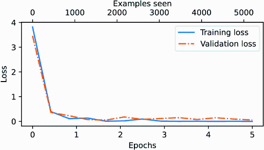
Figure E.5 The training and validation loss curves over six epochs for a machine learning model. Initially, both training and validation loss decrease sharply and then they level off, indicating the model is converging, which means that it is not expected to improve noticeably with further training.
In addition to evaluating the model based on the loss curves, let’s also calculate the accuracies on the full training, validation, and test set (during the training, we approximated the training and validation set accuracies from five batches via the eval_iter=5 setting):
train_accuracy = calc_accuracy_loader(train_loader, model, device)
val_accuracy = calc_accuracy_loader(val_loader, model, device)
test_accuracy = calc_accuracy_loader(test_loader, model, device)

print(f"Training accuracy: {train_accuracy*100:.2f}%")
print(f"Validation accuracy: {val_accuracy*100:.2f}%")
print(f"Test accuracy: {test_accuracy*100:.2f}%")
The resulting accuracy values are
Training accuracy: 100.00%
Validation accuracy: 96.64%
Test accuracy: 98.00%
These results show that the model performs well across training, validation, and test datasets. With a training accuracy of 100%, the model has perfectly learned the training data. However, the slightly lower validation and test accuracies (96.64% and 97.33%, respectively) suggest a small degree of overfitting, as the model does not generalize quite as well on unseen data compared to the training set. Overall, the results are very impressive, considering we fine-tuned only a relatively small number of model weights (2.7 million LoRA weights instead of the original 124 million model weights).